1D Slab Models¶

Vertical slab model¶

To explore the effect of the interplay of dust and line optical depths on the emission spectra, a 1D vertical slab model based on radiative transfer solution is explained here. Figure 1 shows the grid structure adopted for a vertical 1D slab model. This is basically a grid of 0D slab models stacked vertically on top of each other. We apply the LTE radiative transfer equation (Eq. 1) to each slab such that the boundary conditions as shown in the figure are met.

$$\begin{equation} I_{i} = I_{i-1} e^{-\tau_{i}}+S_i(1-e^{-\tau_{i}}) \end{equation}$$

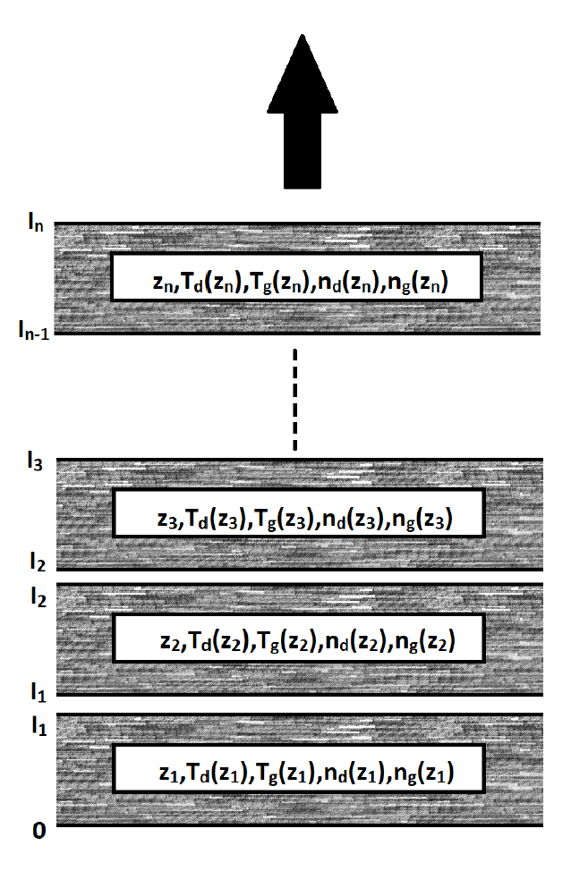Figure 1: 1D vertical slab grid scheme

This gives,

$$\begin{align} I_{1} &= 0+S_1(1-e^{-\tau_{1}})\\ I_{2} &= I_{1} e^{-\tau_{2}}+S_2(1-e^{-\tau_{2}})\\ I_{3} &= I_{2} e^{-\tau_{3}}+S_3(1-e^{-\tau_{3}})\\ I_{n} &= I_{n-1} e^{-\tau_{n}}+S_n(1-e^{-\tau_{n}}) \end{align}$$

Denoting

$$F_i = S_i(1-e^{-\tau_{i}})$$

$$\begin{align} I_{1} &= 0+F_1\\ I_{2} &= I_{1} e^{-\tau_{2}}+F_2\\ I_{3} &= I_{2} e^{-\tau_{3}}+F_3\\ I_{n} &= I_{n-1} e^{-\tau_{n}}+F_4 \end{align}$$

We are only interested in the spectra emitted from the top most slab $n$. So by substitution we get,

$$\begin{equation} I_{n} = F_1e^{-(\tau_{2}+...+\tau_{n})}+ F_2e^{-(\tau_{3}+...+\tau_{n})}+...+ F_{n-1}e^{-\tau_{n}}+ F_n \end{equation}$$

The source function is defined as:

$$\begin{equation} S_i = \frac{j_d(z_i)+\sum_{m=1}^{Nlines}j_g(z_i,m)\phi(z_i,m)}{\kappa_d(z_i)+\sum_{m=1}^{Nlines}\kappa_g(z_i,m)\phi(z_i,m)} \end{equation}$$

where, j is the emission coefficient, κ is the absorption coefficient, ϕ is the profile function, and the subscripts d and g correspond to dust and gas respectively. Numerical implementation:

$$I_n= \begin{pmatrix} F_1 & F_2 & ... & F_{n-1} & F_n \end{pmatrix} \times \begin{pmatrix} e^{-(\tau_{2}+...+\tau_{n})}\\ e^{-(\tau_{3}+...+\tau_{n})}\\ ...\\ e^{-(\tau_{n})}\\ 1 \end{pmatrix}$$

Note that all the flux terms such as I,j,κ,S,F are frequency dependent as well.

The frequency grid upon which this calculation is made should be of high resolving power, R~10^5. This can later be convolved to the required JWST resolution. The following shows an example setup of such a vertical slab model. For the following I assume d=140pc and R=0.1au.

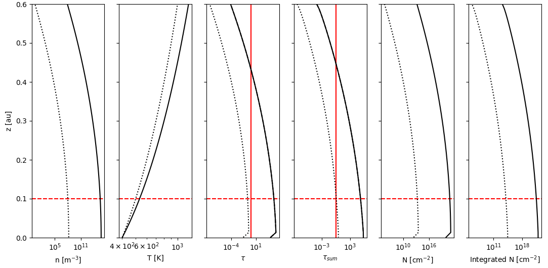Figure 2: dotted: dust, solid: gas, vertical red line is τ = 1 at the wavelength corresponding to the peak of C2H2 spectra. Horizontal dashed lines are the gas and dust scale heights.

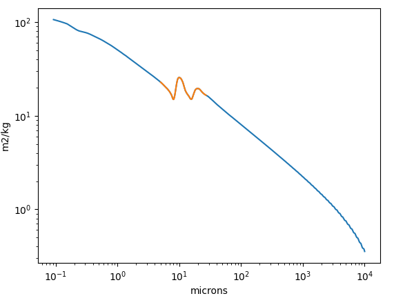Figure 3: Dust opacity used in the model. Directly taken from a standard TTauri ProDiMo model.

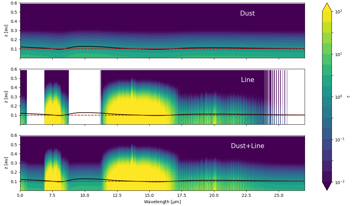Figure 4: Vertically integrated (from the top) optical depth plots. Y axis is the vertical height, X axis is wavelength, the black solid line is the τdust = 1 contour, colorbar shows the optical depths.

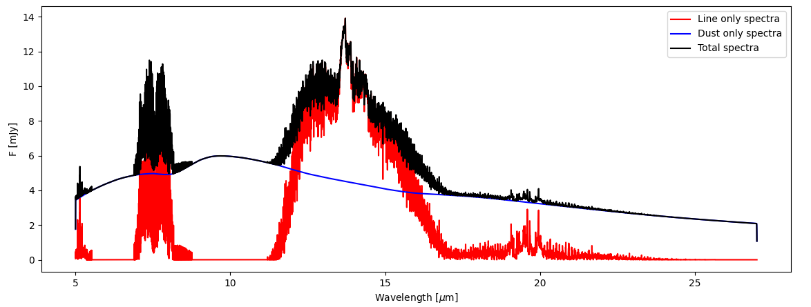Figure 5: Final spectra is show in black, the line only and dust only spectra for the same slab structure are shown in red and blue.

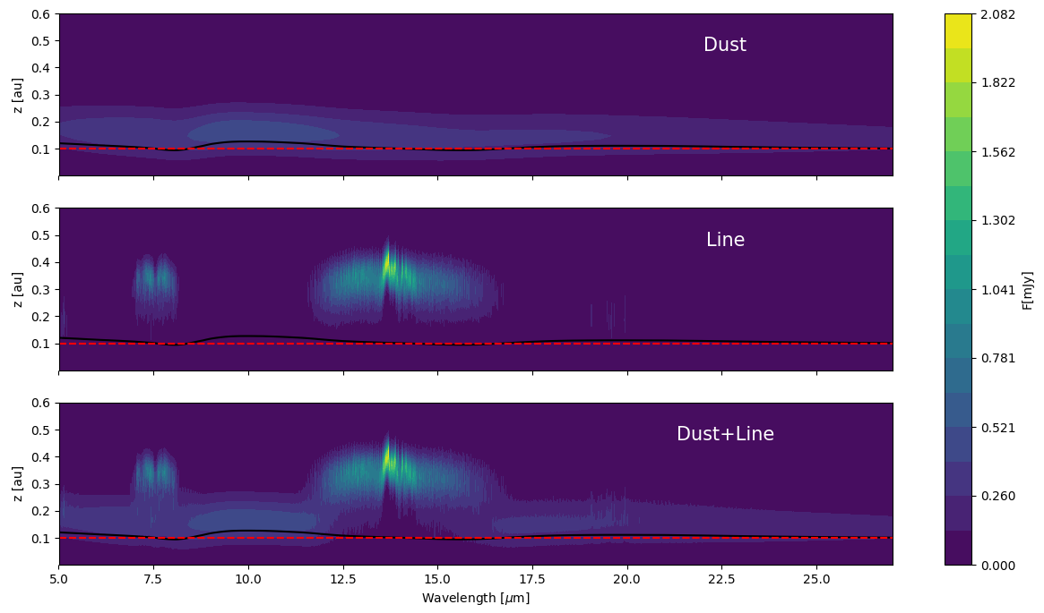Figure 6: Flux contribution of individual slabs (vertical grid points) on a R=105 spectral grid. Red line is the dust and gas scale height. Black line is the τdust = 1 contour.

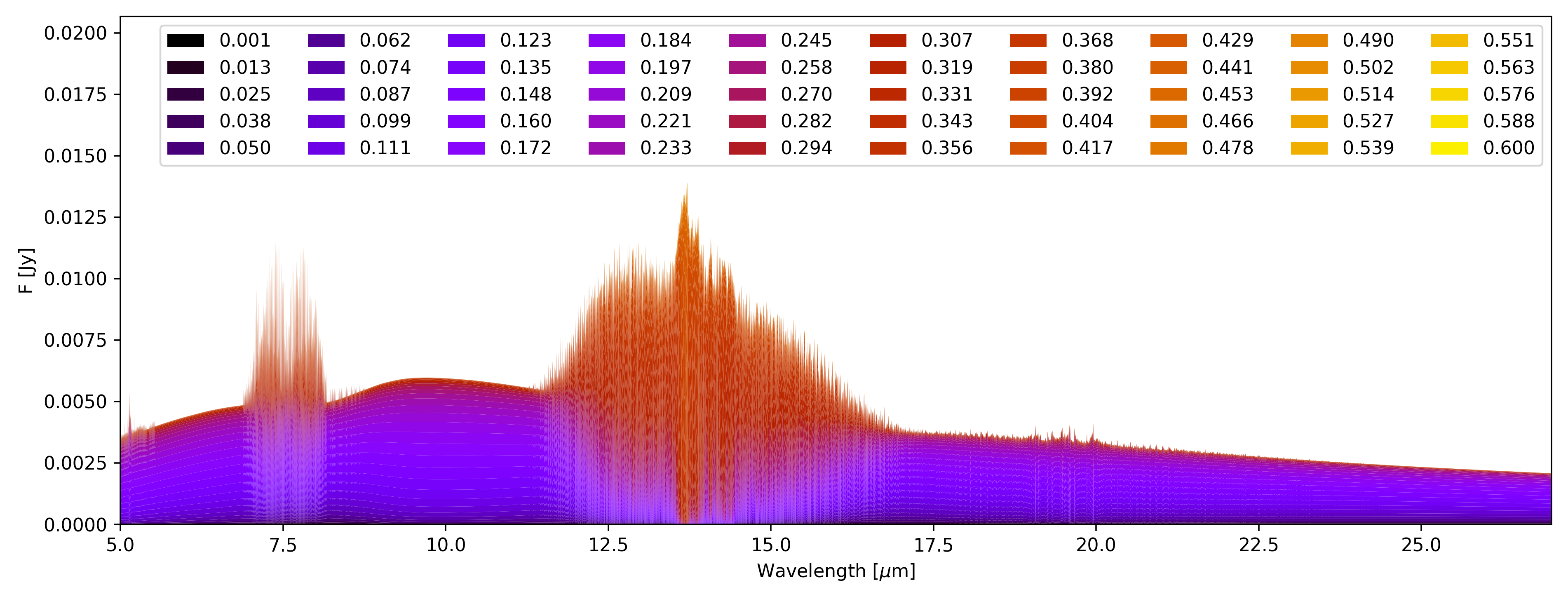Figure 7: Same as previous figure, but contributions stacked on top to build the total spectra.

The main conclusion from such a slab model is that a vertical temperature structure alone cannot reproduce both the molecular continuum and the molecular features of C2H2 observed in J1605 and ISO Cha 147. This is because independent of the temperature and density of gas in the top most slab, the gas emission from rest of the lower slab will need to pass through the top most slab and will be extincted by its optical depth. Since the slab reaches optical saturation well below the top slab, any additional hot gas layer added on top will lead to a balance of further extinction of emission from the bottom by the top layer and equivalent emission of flux from the top layer so as to maintain the blackbody saturation limit. This can be analytically explained by Eq. 10. If we have a slab model with emission $I_n$,

$$\begin{equation} I_{n} = F_1e^{-(\tau_{2}+...+\tau_{n})}+ F_2e^{-(\tau_{3}+...+\tau_{n})}+...+ F_{n-1}e^{-\tau_{n}}+ F_n \end{equation}$$

If we add another layer on top of this $n+1$, then the emergent flux would be, $I_{n+1}$,

$$\begin{align} I_{n+1} &= I_ne^{-\tau_{n+1}}+F_{n+1}\\ I_{n+1} &= F_1e^{-(\tau_{2}+...+\tau_{n}+\tau_{n+1})}+ F_2e^{-(\tau_{3}+...+\tau_{n}+\tau_{n+1})}+...+ F_{n-1}e^{-\tau_{n}+\tau_{n+1}}+ F_ne^{-\tau_{n+1}}+F_{n+1} \end{align}$$

Thus, all the fluxes for i<n+1 are extincted by the optical depth of $n+1$ and the emission from this top layer is determined by $F_{n+1}=S_{n+1}(1-e^{-\tau_{n+1}})$. Alternatively, the additional flux can be written as:

$$\begin{equation} \Delta I = I_{n+1}-I_n = (e^{-\tau_{n+1}}-1)I_n + F_{n+1} \end{equation}$$

Using the definition of $F_{n+1}$,

$$\begin{equation} \Delta I = (1-e^{-\tau_{n+1}})(B_{n+1}-I_n) \end{equation}$$

In the optically saturated case, we can assume that $I_n$ is a blackbody, say $B_<n>$. This gives,

$$\begin{equation} \Delta I = (1-e^{-\tau_{n+1}})(B_{n+1}-B_{\left<n\right>}) \end{equation}$$

If ${T_{\left<n\right>}<< T_{n+1}}$, then $\Delta I < 0$ and we see some absorption features on top.

If $T_{\left<n\right>}\sim T_{n+1}$, then $\Delta I \sim 0$.

If $T_{\left<n\right>}>> T_{n+1}$, then $B_{n+1}>>B_{\left<n\right>}$. Thus $\Delta I \sim (1-e^{-\tau_{n+1}})B_{n+1} = F_{n+1}$.

In the latter case, since $B_{n+1}>>B_{\left<n\right>}$, we get in the final flux $I_{n+1}\sim \Delta I\sim (1-e^{-\tau_{n+1}})B_{n+1}$. This is basically a 0D slab model for only the top layer that replaces the whole 1D vertical structure. As we know, a single slab model cannot reproduce both the molecular continuum and the molecular features.

The input files are more or less same as 0D Slab Models. The switch .true. ! slab_1D initiates ProDiMo into 1D slab model mode. The 1D structure (gas+dust temperatures+column densities) should be provided for each model specified in the SlabInput.in. The line selection is same as in typical LineSelection.in. Following shows an example of running two 1D slab models with a single SlabInput.in file.

Example SlabInput.in file:

***********************************************************
*** Input file for slab escape probability with ProDiMo ***
***********************************************************
*** nmodels should follow output_filename ***
Slab_ ! output_filename
.true.    ! fits_op_files 
.true.    ! slab_1D 
2             ! nmodels
-------------------------------------------------------
*** model 1 ***
1D_struct1        ! structure_from_file 
4.0    28.0      ! line_overlap
1e5              ! R_overlap
           ! end
-------------------------------------------------------
*** model 2 ***
1D_struct2     ! structure_from_file 
4.0    28.0      ! line_overlap
1e5              ! R_overlap
           ! end
-------------------------------------------------------

The 1D structure has to be provided in an ASCII file. The format goes like this:

Number of grid points
Number of species
Species 1
Species 2
.
.
.
Species n
GridIndex GridThickness Vturb DustNumberDens DustTemp Species1NumDens Species2NumDens ... SpeciesnNumDens Species1Temp Species2Temp ... SpeciesnTemp nH2 nHI nHII nHe nelec

Example 1D structures: 1D_struct1:

4
2
C2H2_H
C6H6_C
1  1.000e+00  1.400  1.67e-05  500.000  1.670e+03  1.670e+05  500.000  500.000  0.00e+00  0.00e+00  0.00e+00  0.00e+00  0.00e+00  
2  1.000e+00  1.400  1.67e-05  500.000  1.670e+03  1.670e+05  500.000  500.000  0.00e+00  0.00e+00  0.00e+00  0.00e+00  0.00e+00  
3  1.000e+00  1.400  1.67e-05  500.000  1.670e+03  1.670e+05  500.000  500.000  0.00e+00  0.00e+00  0.00e+00  0.00e+00  0.00e+00  
4  1.000e+00  1.400  1.67e-05  500.000  1.670e+03  1.670e+05  500.000  500.000  0.00e+00  0.00e+00  0.00e+00  0.00e+00  0.00e+00  

1D_struct2:

4
2
C2H2_H
C6H6_C
1 1.0 1.4 1.67115e-5 600 1.67115e-08 1.67115e+05 500 500 0 0 0 0 0 
2 1.0 1.4 1.67115e-5 600 1.67115e-08 1.67115e+05 500 500 0 0 0 0 0 
3 1.0 1.4 1.67115e-5 600 3.34115e+08 1.67115e+05 500 500 0 0 0 0 0 
4 1.0 1.4 1.67115e-5 600 3.34115e+08 1.67115e+05 500 500 0 0 0 0 0 

Horizontal slab model¶

The same 1D slab model infrastructure can be used to calculate a 1D horizontal/radial slab spectra. This becomes even simpler to calculate as individual slabs do not interact with other slabs in terms of opacity. However, the temperature and density structure have to be redefined. The following shows the schematic of the horizontal slab model.

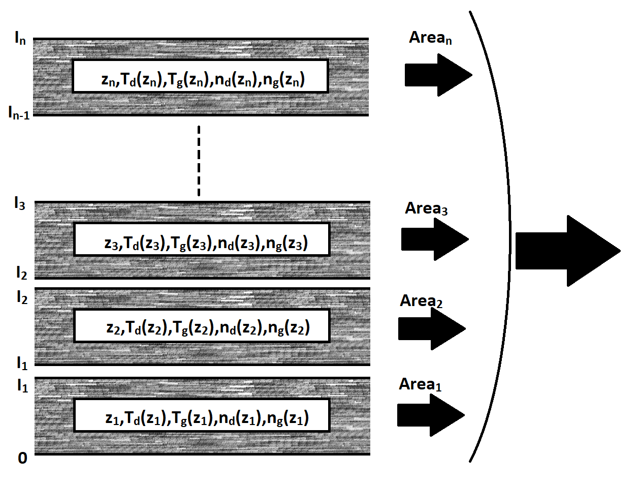Figure 9: Schematic of 1D radial slab model using the same construct as vertical slab model but with necessary changes.

This leads to,

$$\begin{equation} I = \sum_{i=1}^{n} F_i\cdot \Omega_i \end{equation}$$

where, $F_i=(1-e^{-\tau_i})S_i$ and $\Omega_i$ is the emitting solid angle (area).

With such a horizontal/radial slab one can reproduce both molecular continuum and molecular feature of C2H2. Below figure shows the same spectra from the previous section (scaled arbitrarily) in comparison with the radial slab with the same structure.

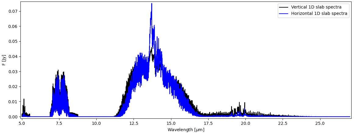Figure 10: Comparison of horizontal and vertical slab model spectra. The fluxes have been arbitrarily scaled for visualization.

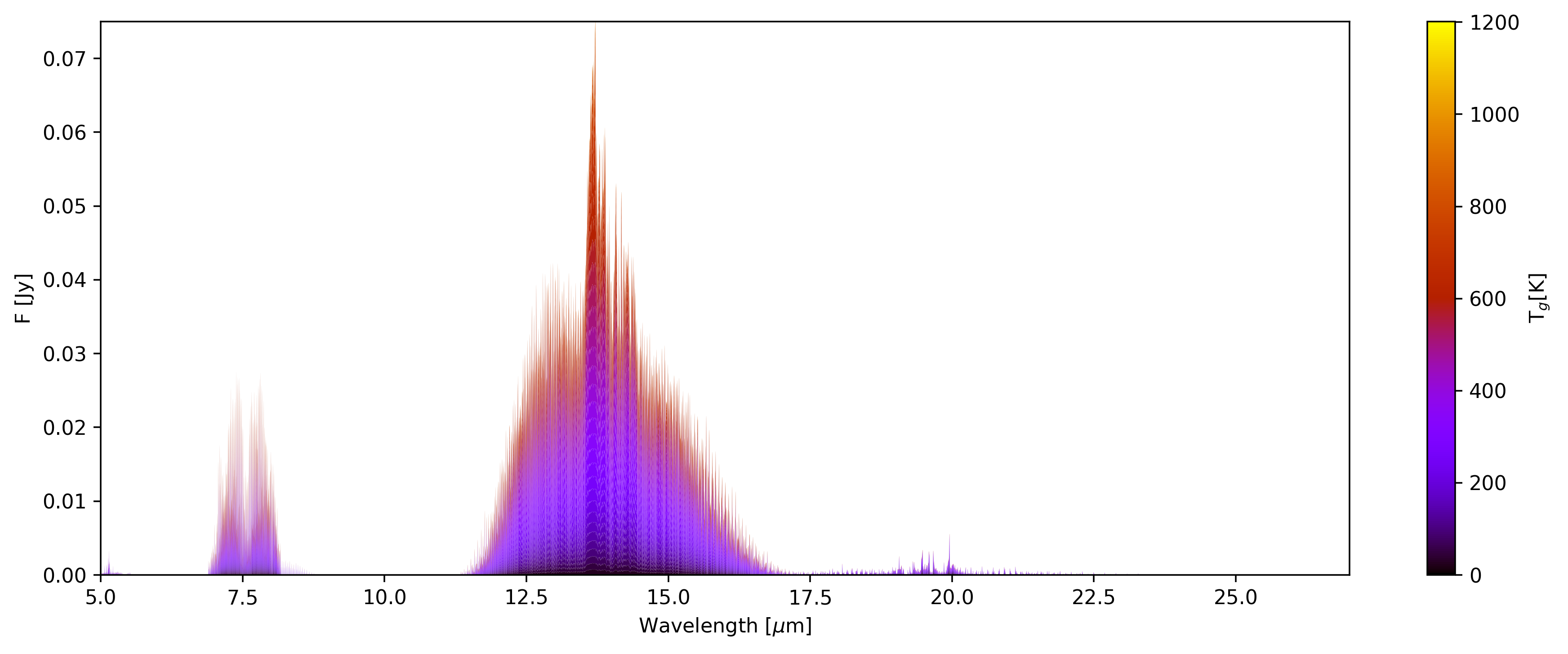Figure 11: Contribution of grid points at different temperature to the final spectra.

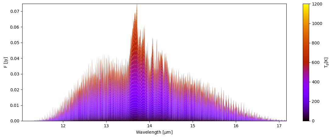Figure 12: A zoom-in of the same figure above.

In terms of input files and switches there is no difference in running a horizontal slab since the calculations hardly differ. Also, ProDiMo only produces output related to vertical slab. Prodimopy should be used to convert a vertical slab into a horizontal slab.