Molecular Cloud models
ProDiMo can run zero-dimensional chemical models of molecular clouds. The option has main purposes:
- create the initial abundances for a time-dependent chemistry in a disk model.
- test chemical networks.
For that many options are available to run the chemistry in addition to the one asking ProDiMo not to run the disk model
To simple run a single molecular cloud model, one simple need to set Parameter.in file:
.true. ! mc_onlyIn that case a time-dependent single point model iwth Tgas=Tdust is run. This is the default for the mc option. Further flags related to a molecular cloud run for 'Parameter.in' can be found in How_to_run_a_time_dependent_chemistry_model.
Further options exist:
- Tgas=Tdust but at steady-state (addtionally to mc_only)
.true. ! mc_steady_state- The chemistry is at steady-state but Tgas is obtained by balancing the heating and the cooling
.true. ! mc_thermal_balanceFor further otions set the section Running a grid of molecular cloud models.
Setting the dust parameters
Setup Parameter.in with only one type of bare grains and without settling (to avoid unnecessary slow computations). For example:
------ dust parameters ------
2.094       ! rho_gr      [g/cm^3]: dust grain material mass density
0.05        ! amin        [mic]   : minimum dust particle size
3000.0      ! amax        [mic]   : maximum dust particle size
3.5         ! apow        [-]     : dust size distr f(a)~a^-apow
dust_opacity_list2.txt            ! dust_opacity_list_file
3           ! NDUST               : number of selected dust species
  0.60      Mg0.7Fe0.3SiO3[s]
  0.15      amC-Zubko[s]
  0.25      vacuum[s]
Running a grid of molecular cloud models
There is a possibility to run a grid of Molecular Cloud models (the source is in time_dependent_mc.f)
.true. ! mc_gridTo request a grid of models, one needs a supplementary input file named Molecular_Cloud_Input.in. An example is given in the directory ../input_examples/molecular_clouds/ together with a Parameter.in file showing the way to run a grid of models. The clouds parameters in both Parameter.in (for one unique model) or in Molecular_Cloud_Input.in are (The format of the input is the same than for Parameter.in).
-----------------------------------------------------------------
3            ! nmodels           : number of molecular cloud models
0            ! verbose_level     : how much output? (-1...4)
---------------------------------------------------------------
*** Run the default TMC-1 model at steady-state
test_mc1_large.out ! model_filename       : use defaul TMC-1 parameters
.true.       ! mc_steady_state
.false.      ! mc_thermal_balance
.true.       ! end                  : obligatory at the end of each model description
---------------------------------------------------------------
*** Example of how to run a model at steady-state with thermal balance
test_mc2_large.out ! model_filename : output filename
1e6         ! nH_mc    : molecular cloud number density in cm^-3
20.          ! Td_mc     : dust temperature in K
20.          ! Tg_mc     : gas temperature in K initial guess  (in case of thermal balance calculations)
100.0      ! CHI1_mc : UV field in band 1
100.0      ! CHI2_mc : Uv field in band 2
0.1          ! a1_mc : grain mean radius in micron
0.01        ! dust_to_gas_mc
3.0          ! rho_gr_mc
0.2          ! vturb_mc [km/s]
10.0        ! Av_mc             : extinction to the edge of the cloud
.false.      ! mc_steady_state
.true.       ! mc_thermal_balance : compute the abundances together with the thermal balance
.true.       ! end                : required parameter
---------------------------------------------------------------
*** Example of parameters to run a time-dependent cloud model for different age output
DIANA_large.out ! model_filename
1e6          ! nH_mc    molecular cloud number density in cm^-3
20.          ! Td_mc    dust temperature in K
20.          ! Tg_mc    gas temperature in K initial guess
100.0        ! CHI1_mc
100.0        ! CHI2_mc
0.01         ! dust_to_gas_mc
3.0          ! rho_gr_mc
0.2          ! vturb_mc [km/s]
10.0         ! Av_mc      : cloud extintion
48            ! N_age_mc : number of age bins (the ages are give in the next line in years)
1e2 5e2 1e3 2e3 3e3 4e3 5e3 6e3 7e3 8e3 9e3 1e4 2e4 3e4 4e4 5e4 6e4 7e4 8e4 9e4 1e5 2e5 3e5 4e5 5e5 6e5 7e5 8e5 9e5 1e6 2e6 3e6 4e6 5e6 6e6 7e6 8e6 9e6 1e7 2e7 3e7 4e7 5e7 6e7 7e7 8e7 9e7 1e8
.false.      ! mc_steady_state
.false.      ! mc_thermal_balance
.true.       ! end
Every line starting with - or * are considered as a comment line. An example of the output file in prodimo.log
...
**********************************
 Molecular chemistry grid of models

 Molecular cloud model            1
 Call molecular cloud chemistry solver

 Computing molecular cloud abundances ...
        cloud lifetime [yrs] = 1.700E+05
  gas number density [cm^-3] = 1.000E+04
             dust size [mic] = 1.000E-01
 dust number density [cm^-3] = 1.854E-08
   cloud gas temperature [K] = 1.000E+01
  cloud dust temperature [K] = 1.000E+01
  UV CHI1                    = 1.000E+00
  UV CHI2                    = 1.000E+00
  AV                         = 1.000E+01
 Computing rate coefficients for ISM environment ...
 Steady-state chemistry ...
 Steady solver failed. Use initial guess from advanced chemistry
 Success...
 Model filename=test_mc1_large.out

 Molecular cloud model            2
 Call molecular cloud chemistry solver

 Computing molecular cloud abundances ...
        cloud lifetime [yrs] = 3.000E+06
  gas number density [cm^-3] = 1.000E+06
             dust size [mic] = 1.000E-01
 dust number density [cm^-3] = 1.854E-06
   cloud gas temperature [K] = 2.000E+01
  cloud dust temperature [K] = 2.000E+01
  UV CHI1                    = 1.000E+02
  UV CHI2                    = 1.000E+02
  AV                         = 1.000E+01
 Molecular cloud with thermal balance ...
   cloud gas temperature [K] = 2.000E+01
 Model filename=test_mc2_large.out

 Molecular cloud model            3
 Call molecular cloud chemistry solver

 Computing molecular cloud abundances ...
  gas number density [cm^-3] = 1.000E+06
             dust size [mic] = 1.000E-01
 dust number density [cm^-3] = 1.854E-06
   cloud gas temperature [K] = 2.000E+01
  cloud dust temperature [K] = 2.000E+01
  UV CHI1                    = 1.000E+02
  UV CHI2                    = 1.000E+02
  AV                         = 1.000E+01
 Computing rate coefficients for ISM environment ...
 Advance_chemistry for mol.cloud parameters ...
        cloud lifetime [yrs] = 1.000E+02
        cloud lifetime [yrs] = 5.000E+02
        cloud lifetime [yrs] = 1.000E+03
        cloud lifetime [yrs] = 2.000E+03
        cloud lifetime [yrs] = 3.000E+03
        cloud lifetime [yrs] = 4.000E+03
        cloud lifetime [yrs] = 5.000E+03
        cloud lifetime [yrs] = 6.000E+03
        cloud lifetime [yrs] = 7.000E+03
        cloud lifetime [yrs] = 8.000E+03
        cloud lifetime [yrs] = 9.000E+03
        cloud lifetime [yrs] = 1.000E+04
        cloud lifetime [yrs] = 2.000E+04
        cloud lifetime [yrs] = 3.000E+04
        cloud lifetime [yrs] = 4.000E+04
        cloud lifetime [yrs] = 5.000E+04
        cloud lifetime [yrs] = 6.000E+04
        cloud lifetime [yrs] = 7.000E+04
        cloud lifetime [yrs] = 8.000E+04
        cloud lifetime [yrs] = 9.000E+04
        cloud lifetime [yrs] = 1.000E+05
        cloud lifetime [yrs] = 2.000E+05
        cloud lifetime [yrs] = 3.000E+05
        cloud lifetime [yrs] = 4.000E+05
        cloud lifetime [yrs] = 5.000E+05
        cloud lifetime [yrs] = 6.000E+05
        cloud lifetime [yrs] = 7.000E+05
        cloud lifetime [yrs] = 8.000E+05
        cloud lifetime [yrs] = 9.000E+05
        cloud lifetime [yrs] = 1.000E+06
        cloud lifetime [yrs] = 2.000E+06
        cloud lifetime [yrs] = 3.000E+06
        cloud lifetime [yrs] = 4.000E+06
        cloud lifetime [yrs] = 5.000E+06
        cloud lifetime [yrs] = 6.000E+06
        cloud lifetime [yrs] = 7.000E+06
        cloud lifetime [yrs] = 8.000E+06
        cloud lifetime [yrs] = 9.000E+06
        cloud lifetime [yrs] = 1.000E+07
        cloud lifetime [yrs] = 2.000E+07
        cloud lifetime [yrs] = 3.000E+07
        cloud lifetime [yrs] = 4.000E+07
        cloud lifetime [yrs] = 5.000E+07
        cloud lifetime [yrs] = 6.000E+07
        cloud lifetime [yrs] = 7.000E+07
        cloud lifetime [yrs] = 8.000E+07
        cloud lifetime [yrs] = 9.000E+07
        cloud lifetime [yrs] = 1.000E+08
 Model filename=DIANA_large.out
...
Analyzing and plotting the results
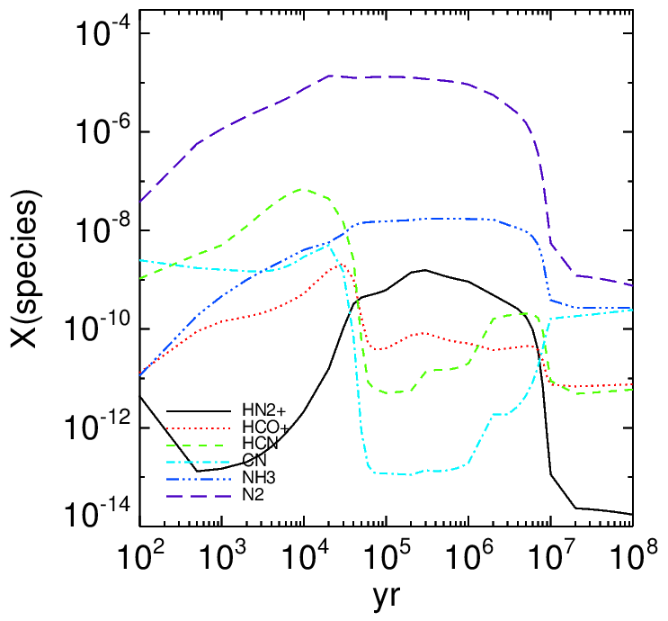
The chemical abundances are in the files with names provided in the supplementary input file (example test_mc1.out) Plots of the time-dependent runs can be made using the IDL program analyse_time_dependent_clouds.pro (in /input_example/molecular_cloud/).
IDL > analyse_time_dependent_clouds,'DIANA_large.out','DIANA_large.ps',1e2where DIANA_large.out is the output file given in the Molecular_Cloud_Input.in file. DIANA_large.ps is the name of the figure output file, and 1e2 is the smallest time to be plotted in years (here is 100 years). An example is given below (, , , ).
Alternatively, one can use a python script in ../python
python3 MolCloud_SurfChem.pyPython version 3 is supported. The list of species to be plotted are hard-coded in the script. So one has to change the code to suit the molecules to be displayed (molecules listed in the python script that are not included in the model are interpreted as "0", drawing a log(0) error when plotted). A quick description of the routine usage can be obtained by typing
python3 MolCloud_SurfChem.py -hSetting initial abundances
It is also possible to start the molecular cloud run from an abitrary set of initial abundances. This can be done in the same way as for a time-dependent disk model and ist described here. The only difference is that the flag for the initial abundances in Parameter.in is
Restart using previous abundances
Restarting from a previously computed Molecular_cloud.out file. Add the two following lines in the Molecular_Cloud_Input.in file
Molecular_cloud.out ! previous_mc_model_filename
.true.              ! start_from_previous_mc_model
Limitations on the time step
time step for ages < 1e7 yrs are restricted to a maximum step of 1 Myrs (1e6 yrs). Beyond 1e7 yrs, one can choose arbitrary time steps
Diffuse X-ray background
from 30 sept 2015, one can model X-ray gas-phase reactions using the flag in Molecular_Cloud_Input.in
1e-5 ! Xray_Lum_mc in erg/sThen the full X-ray chemistry treatment of ProDiMo is used.
Choice of ODE solvers
One can choose different stiff ODE solvers. GEAR is a very old method that has been superseded but still available for benchmark. LSODE replaces GEAR, it is more efficient. DVODE is the most efficient all-usage routine. It is comparable or faster than the LIMEX solver, which is the default solver used in ProDiMo. We included two solvers from the numerical recipes book (you should only use them if you have the book): ROSEN and STIFBS. The flags are set in Parameter.in
.true. ! ROSEN
.true. ! STIFBS
.true. ! DVODE
.true. ! GEAR
.true. ! LSODE
H2, C, and CO (self)-shielding
from revision e9ebf29f, the code will estimate the H2, C, and CO shielding based on the density, UV field, gas temperature and Av. The scaling laws are derived from PDR models where the Av thresholds for shielding is known to vary as Go/(n*sqrt(Tg)). The default values are AV_H2_mc = 0.5, AV_C_mc =1.0, and AV_CO_mc = 3.0. In Molecular_Cloud_Input.in, one can change those values:
0.5    ! AV_H2_mc
1.0    ! AV_C_mc
3.0    ! AV_CO_mc
Those shielding helps the build-up of those species, especially in models with low Av. The screen output now includes estimates of N(H2), N(C), and N(CO), which are used in the (self-shielding) formula in ProDiMo.
 Computing molecular cloud abundances ...
 gas number density [cm^-3]  = 2.000E+05
 dust size [mic]             = 1.000E-02
 dust number density [cm^-3] = 3.708E-04
 dust albedo (albedoUV)      = 6.000E-01
 cloud gas temperature [K]   = 1.000E+01
 cloud dust temperature [K]  = 1.000E+01
 UV CHI1                     = 1.000E+00
 UV CHI2                     = 1.000E+00
 AV                          = 1.000E+01
 estimated N(H2) [cm^-2]     = 9.492E+21
 estimated N(C) [cm^-2]      = 6.197E+15
 estimated N(CO) [cm^-2]     = 1.891E+18
 PDR scaling factor          = 1.581E-02
 Cosmic Ray ion rate [s^-1]  = 1.360E-17
The PDR scaling factor is 1e4*CHI1_mc/nH_mc/sqrt(Tg_mc), ie for 1e3 cm-3, 100 K and 1 ISM UV, it is equal to 1.
Alternative chemicaldesorption law
from revision e9ebf29f, it is possible to use the formula for surface chemistry chemical desorption described in Minissale et al. 2015 [http://arxiv.org/abs/1510.03218]. The switch in Parameter.in is
.true. ! Minissale_evapThe default is the usage of the Rice Rampsberger Kassel model. Holbrook, Piling, & Robertson 1996 Unimolecular Reactions, 2nd ed, Wiley Ney-York, and Garrod & Herbst 2006.