Code performance optimizations¶

2021-12-202025-10-20

Flags affecting speed and stability of chemistry (07/2024)¶

.true.      ! quadp_solver       : enable quadruple precision chemistry solver?
20.0        ! cputime_max [s]    : max. wall clock time for advance_chemistry 
.true.      ! chem_stability     : allow extending time interval beyond 1.E+7 yrs
0           ! numerical_jacobian : use numerical rather than analytical Jacobian?
.true.      ! NewChemScan        : new initial concentrations from down-right scan?
.false.     ! use_chemsol        : use a database of chemical solutions to guess init.conc.
1.0E-6      ! temp_precis        : rel. precision in T-determination
1.0E-8      ! chem_precis        : rel. precision in solve_chemistry

(the values listed above are the ProDiMo v3 default values).

Before explaining the effects of these flags, we need to understand ProDiMo's strategy to solve the t-independent chemistry. The basic solution method is Newton-Raphson (NR), with linear back-paddling in case an iteration resulted in a worse result, which is called PULLBACK in the code. Having a precise and fast Jacobian, which points the way towards the solution, is the key to accelerate ProDiMo.

This method alone, however, in double precision, often fails because we start the iterations with initial concentrations that are simply too far away from the final solution. Problems occur, in particular, at the main chemical phase transitions, such as H -> H2, C+ -> C -> CO, H2O -> H2O# etc., where suddenly all concentrations change by orders of magnitude. Therefore, ProDiMo uses a certain sequence of actions and solution methods to get to the solution anyway.

Try the standard double-precision NR method with analytic Jacobian (maxit=100 iterations max)
If numerical_jacobian>0 is selected, switch to double-precision NR method with numerical Jacobian after maxit/2
If the conditional number of the Jacobian matrix indicates that the matrix cannot be inverted with double precision arithmetic, change to quadruple precision after 30 iteration (if quadp_solver=T)
If numerical_jacobian>0 is selected, switch to quad-precision numerical Jacobian after half of the remaining iterations
If everything failed so far, advance the chemistry to tend = Min{100 tau_chem, 1.E+7 yrs}, where the chemical relaxation timescale tau_chem is estimated in GUESS_TAUCHEM. The time-integration will stop, however, once the wall clock time exceeds cputime_max.
If tend is reached, and wall clock time is still < cputime_max/10, and chem_stability=T, extend tend by factor 3 and go back to step 5.
Based on the now (hopefully much) improved concentrations after advancing the chemistry (steps 5+6), repeat steps 1-4 for maxit=200 iterations (60 when the quadruple solver is used again).

Another important issue for code speed and stability is how the initial concentrations (before step 1) are estimated, which is done in routine GUESS_CHEMISTRY, realising that many subsequent chemistry calls will be necessary to determine the temperature. When a new point is started, the standard strategy (NewChemScan=T) is to take the concentrations from the finished point above. Another idea is to set use_chemsol=T, in which case ProDiMo automatically builds up a database of chemical solutions as function of $n_\mathrm{<H>}$ , $T_\mathrm{g}$ and $A_\mathrm{V}$ , and improves that database with every call.

A new acceleration idea (since 07/20224) is to save not only the concentrations for the subsequent chemistry calls, but also the successful solution method used, so that in the next call, ProDiMo can skip some of the steps 1-3, and apply that successful solution method immediately.

Another remark concerns the setting of the relative tolerances chem_precis and temp_precis. It is very important to have temp_precis >> chem_precis, otherwise, if chemical concentrations are allowed to randomly vary by chem_precis in subsequent calls, the heating and cooling rates will do so, too, and finding a temperature solution within temp_precis is likely impossible, which will result in an endless series of chemistry calls, trying to resolve the randomness ...

If you are running standard small chemistry models, it is probably OK to use the standard setups as above. However, if you use larger networks and/or surface chemistry and/or STAND2020 with reaction inversions and/or extended chemistry like Jayatee Kanwar's hydro-carbon chemistry, and observe a lot of "t", "T" or "#" in the logfile, you might want to try the following:

try larger cputime_max. This allows for longer integration times in steps 5 and 6, resulting in better guesses for step 7. Once a proper t-independent solution is found, subsequent calls will be much faster! Time for matrix operations scales as N³. If your chemistry has N=300 species (large DIANA standard is 200), well, then use 20sec x (N/200)³ = 67sec.
try chem_stability=T. Again, this might enable ProDiMo to find solutions that are impossible to find otherwise.
try use_chemsol=T, and run such models several times!
make sure that temp_precis >> chem_precis

The exact meaning of the integer numerical_jacobian is as follows

0: no use of numerical Jacobians
1: use numerical Jacobians after some time in SOLVE_CHEMISTRY
2: as 1, but also use the same numerical Jacobians in ADVANCE_CHEMISTRY (not recommended)
3: as 1, but also use the inbuilt numerical Jacobians of the ODE solvers in ADVANCE_CHEMISTRY

The usage of numerical_jacobian=1 is not really recommended, it has rather been implemented to check whether the analytical Jacobian is correct.

Accelerating ProDiMo (slightly outdated - but still valid!)¶

Is ProDiMo too slow?

The first (obvious) option to accelerate it, is to use a smaller spatial grid, the CPU time roughly scales with (Nx * Nz).
TODO: This is likely not working any more, only with a particular MCFOST version. The next option is NOT to use ProDiMo for the continuum radiative transfer, but run MCFOST or MCMAX, and then run ProDiMo on top of these results, see ProDiMo <-> MCFOST.
You can decrease the selection of chemical species, the chemistry-part of the code scales roughly with $\mathrm{Nsp}^3$ .
You can compile and use an OpenMP parallel version, see Parallel ProDiMo, which results in an acceleration that depends on the number of processors (more precisely on the number of cores).
You should compile with -O3 flag (acceleration factor ~3), but avoid -fast which has impact on precision, actually causing the code to not converge and slow down
You can try faster linear algebra libraries (openblas or mkl), see Blas_Lapack, maybe 30%.
NEW (15.08.2013) You can use flag use_chemsol = .true. in Parameter.in. First tests look promising, and result in an acceleration of about 40%. The idea is to store all chemical results in a database in { $A_\mathrm{V}$ , $n_\mathrm{\left<H\right>}$ , $T_\mathrm{gas}$ , $T_\mathrm{dust}$ }, and then start the chemical iterations from the closest solution in the database.

When you first run it, ProDiMo will not be faster, it will create (and start to use) a database called chemsol.dbase. In subsequent runs of the same or very similar disk setups, you should then observe an acceleration. With a bit of luck, this procedure also removes some artefacts from the midplane, where finding the chemical kinetic equilibrium solution is very difficult. By using the database, the non-converging points are successively advanced in time with every run, properly converged points are preferentially taken as starting values, and ProDiMo preferentially takes the CO-poor solutions in the midplane as starting points. Note that, therefore, the results will not be 100% reproducible.

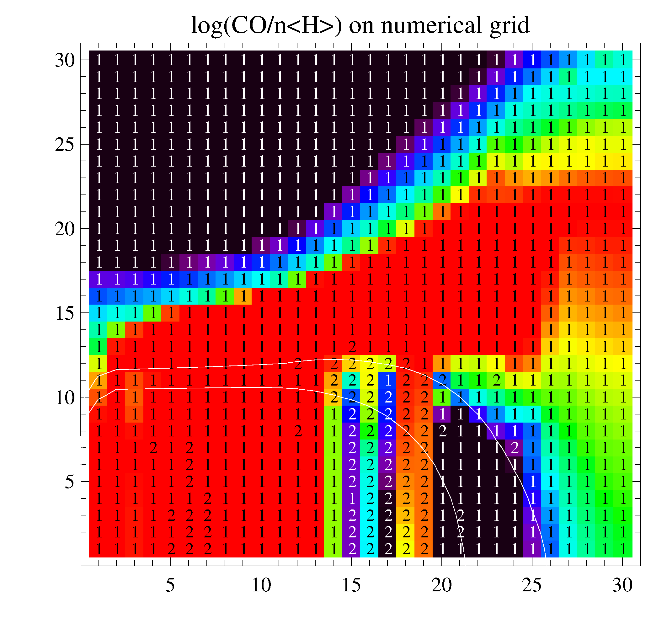
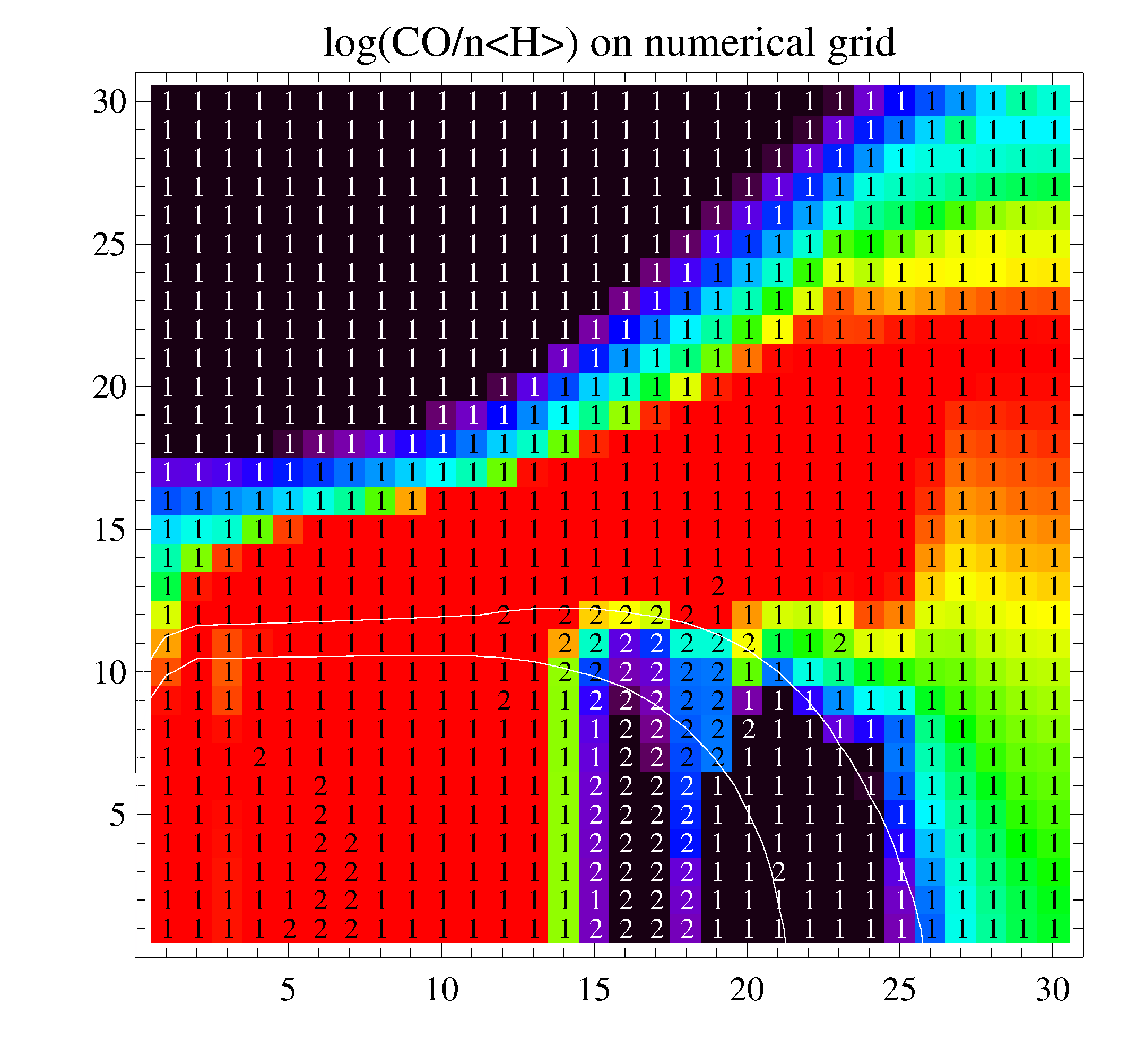
The two figures show the calculated CO-concentrations on the numerical grid. L.h.s. is without using the database, r.h.s. is after three runs using the database. The labels have meanings as "1"->kinetic equilibrium and "2"->time-dependent solver used for 1.E+7 years. The test was computed with a large selection of 162 species and 2233 reactions (X_rays, PAHs, 28 ices). The problematic region is below Av=10, between the H2O and CO ice lines, where for t->oo, CO is very slowly dissociated by cosmic rays, and disappears in form of H2O# ice, creating a carbon-rich chemistry with organic molecules in the midplane. The integration time of 1.E+7 yrs for the advance-solver is too short to reveal this behaviour.
NEW (16.08.2013) You can ignore the gas energy balance in the midplane, and assume Tgas=Tdust in the midplane instead, by saying ignore_Tg_midplane. With this option, ProDiMo will not determine the gas temperature if
- $min(A_\mathrm{V,ver},A_\mathrm{V,rad})>10$ and if
- $|1-T_\mathrm{gas}(ix,iz+1)/T_\mathrm{dust}(ix,iz+1)|<0.01$
This seems to work really well, my tests show quite acceptable changes in the computed line fluxes: E-18-fluxes < 0.1%, E-19-fluxes < 1% (however, NH3-lines are tricky <15%), at an acceleration of a factor of roughly 2.

The following table summarizes the test results for a small 30x30 model ("ParallelTest") with big chemistry (162 species, 2233 reactions). The chemsol.dbase is well relaxed, and overwritten by a copy before each run. I was using 6 CPUs for the parallel runs.

 parallel_chem | use_chemsol | ignore_Tg_midplane | user-time[sec]
 -----------------------------------------------------------------
    .false.    |   .false.   |      .false.       |    581.89
    .false.    |   .false.   |      .true.        |    295.92
    .false.    |   .true.    |      .false.       |    360.84
    .false.    |   .true.    |      .true.        |    149.11
    .true.     |   .false.   |      .false.       |    170.43
    .true.     |   .false.   |      .true.        |     82.42
    .true.     |   .true.    |      .false.       |    105.43
    .true.     |   .true.    |      .true.        |     42.04

The net effect of all 3 ideas, used simultaneously, is an acceleration of a factor of 13.8 (!), at the expense of deviations in the computed line fluxes of <5%. I checked CO, 13CO, C18CO sub-mm, high-J CO, CO ro-vib, OI 63,145,6300, OH and H2O Herschel lines. As I mentioned above, some lines may be more tricky like NH3.

Note that use_chemsol = .true. will lead to non-reproducible results, and ignore_Tg_midplane is physically not quite the same. Both accelerations can change the results somewhat, but the differences should be small. In particular, combining parallel_chem = .true. with use_chemsol = .true. is expected to destroy the possibility to parallel_debug, because the results will not be 100% reproducible anyway. This is not a bug, but a consequence of the idea of using a chemical solution database, which updates itself on the fly. However, I made some tests which even passed the parallel test (see Parallel ProDiMo).

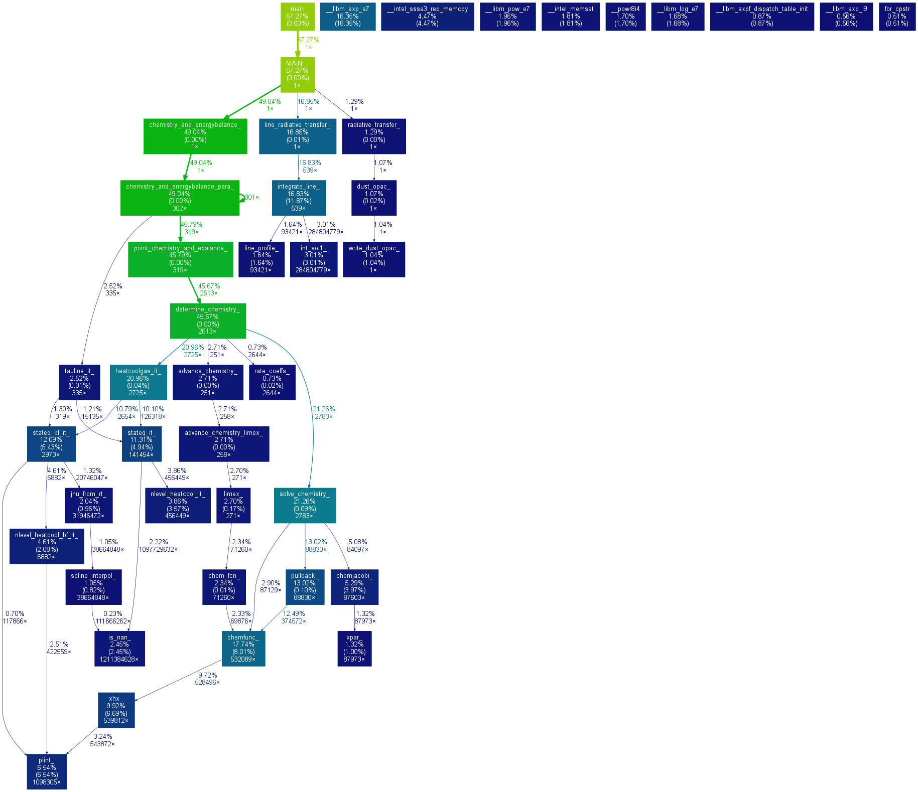
The figure below shows the results of a profiling run in folder "ParallelTest". The code was compiled with ifort with the external mkl library (see Blas Lapack) and run using

  FLAGS = -r8 -i4 -g -traceback -O3 -xHOST -prec-div -fp-model source -qopenmp -p
  FCRIT = -r8 -i4 -g -traceback -O3 -xHOST -prec-div -fp-model source -qopenmp -p

Flags in Parameter.in:

  parallel_chem=T
  Hatom_bb=T
  Hatom_bf=T

Number of threads:

  setenv OMP_NUM_THREADS 6

After compiling with -p option and running, you can use gprof for profiling, and visualize the results as

  gprof ../src_develop/prodimo | ../python/gprof2dot.py | dot -Tpng -o gprof.png

Note that there is no continuum radiative transfer carried out in "ParallelTest". In this configuration, ProDiMo spends most of the time to solve chemical equations (solve_chemistry -> 21%), heating & cooling (stateq_bf_it -> 12%, stateq_it -> 11%), line radiative transfer (->17%) and to compute exponential functions (-> 16%). The chemistry is mostly time limited by routines chemfunc and xhx.

Performance Tests (Compilers)¶

Here are some results from a recent ProDiMo performance test using different compilers. If you really want to fully optimize ProDiMo on your machine/cluster we recommend to do something similar, as the results can be machine dependent.

Laptop = IWF2-065: INTEL-Core-i9-13900  OMP_NUM_THREADS=12
       ifort (IFORT) 2021.10.0 20230609
       ifx Version 2024.0.2 Build 20231213
       -r8 -i4 -O3 -msse4.2 -xHOST -prec-div -fp-model source -qopenmp
       gfortran 11.4.0
       -fdefault-real-8 -fdefault-double-8 -O3 -std=legacy -march=native -fopenmp

PC     = AMD Ryzen Threadripper PRO 3975WX 32-Cores  OMP_NUM_THREADS=32
       ifort (IFORT) 2021.10.0 20230609
       ifx Version 2024.0.2 Build 20231213
       -r8 -i4 -O3 -msse4.2 -xHOST -prec-div -fp-model source -qopenmp
       gfortran 11.4.0
       -fdefault-real-8 -fdefault-double-8 -O3 -std=legacy -march=native -fopenmp

leo18  = AMD EPYC 7542 32-Core Processor  OMP_NUM_THREADS=32
       ifort (IFORT) 19.1.3.304 20200925
       -r8 -i4 -O3 -msse4.2 -xHOST -prec-div -fp-model source -qopenmp
       gfortran 8.5.0 20210514
       -fdefault-real-8 -fdefault-double-8 -O3 -std=legacy -march=native -fopenmp

                      ------Laptop-------   ---------PC--------   ---leo18----
                      ifort    ifx  gfort   ifort    ifx  gfort   ifort  gfort
       INIT time[s] =    14     14     16      10     21     21      38     27
   RT total time[s] =   408    387    348     232    199    181     286    345
        SED time[s] =     6      6      8       4      4      7       5      9
  chemistry time[s] =   586    631    685     445    458    405     601    605
      quadp,advance = 891,40 890,56 900,47  891,54 920,71 906,43  896,53 904,48
         RT time[s] =   172    167    162      71     64     60      82     80
-------------------------------------------------------------------------------
  total CPU time[s] = 13345  13679  12887   21576  21156  12110   27268  19754
  total usertime[s] =  1200   1218   1236     797    767    700    1039   1113

Parallel performance and number of threads¶

Christian Rab has performed some tests (Jan 2024) to help the user choose the appropriate number of threads (see setup your OS environment) to run a typical ProDiMo model. Many of the details of the conclusion will depend on the actual model. In particular, the chemical solver is very sensitive to the number and types of species.

Setup¶

cluster node with 72 cores (not the same node, but the should be essentially the same).
Change OMP_NUM_THREADS using 1, 2, 4, 8, 16, 32, 64, 72 and run a model for each
The standard T Tauri model from the examples directory is used. With 100x100 grid points, 100 RT iterations and increased the number of grid points for line RT. All other parameters unchanged
Mie.fits.gz and escape-probability tables are already there. with this setup, the runtime is mostly dominated by the continuum RT
used ProDiMo version 3.0.0
compiled with ifort version Version 2021.4.0 (no EXTERNAL_LAPACK)

Results¶

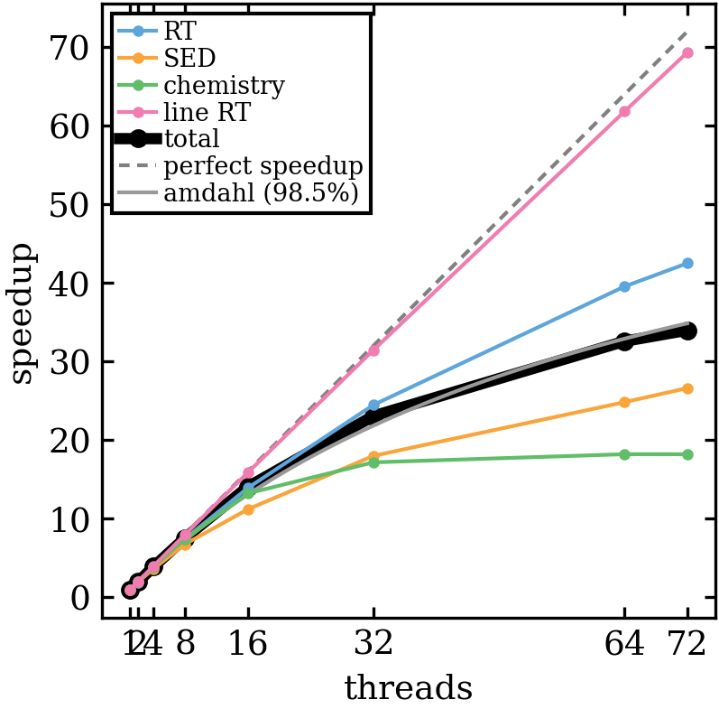
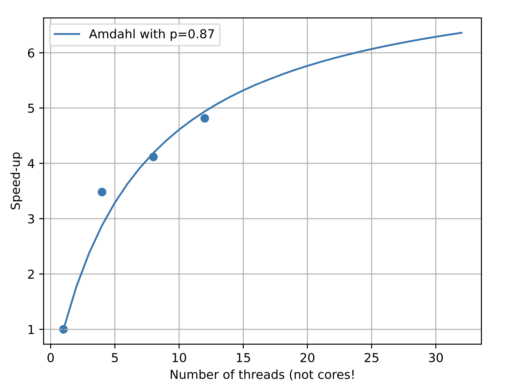
Speedup figure: total is the speed-up considering the total runtime (taken from finished.out). Applying Amdahls law would mean a parallel fraction of about 98.5%. Other lines are self-explanatory I would say.
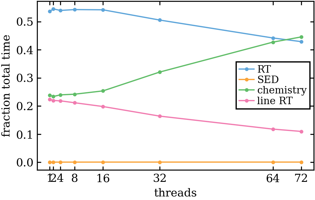
Fraction of total time figure: This gives the fraction of the time spent in the RT (continuum), SED chemistry and line RT parts. For the chemistry, there is no speed-up for threads > 32 any more so it becomes the slowest part at some point.
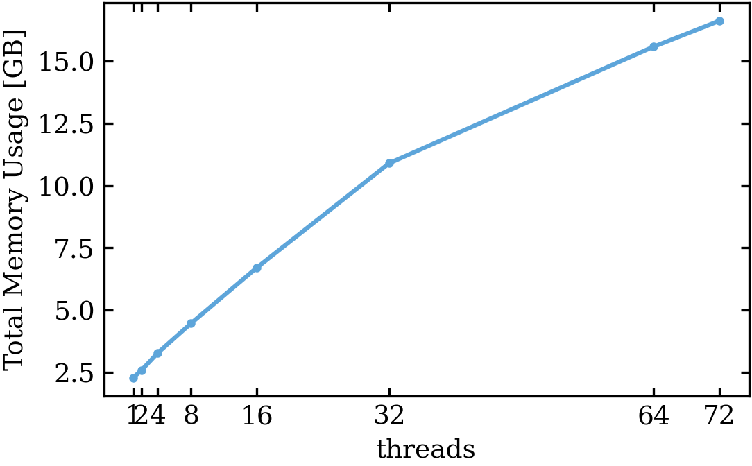
Total memory usage figure: : This number I also get from the slurm system. This should be the max memory used during the model runtime. just for your information, those nodes have 264 GB of ram for reference: the total runtime for the one-thread model was 21 h 46 m 45 s, for the model with 72 threads, it was 0 h 38 m 34 s.
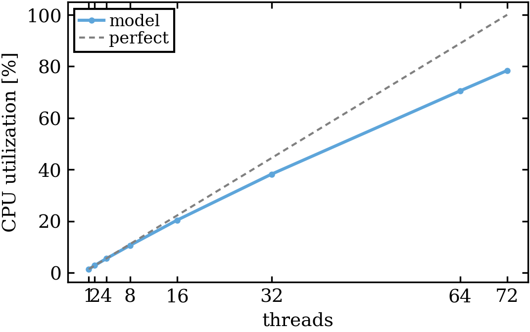
CPU utilization figure: Indicates how much of the available CPU power was used during the model runtime.


	$fraction_time$

Gfortran tests¶

Using the gfortran compiler on a Mac 8 cores (16 threads) machine. Only the chemistry part has been tested

prodimo_chemistry_speedup

Some conclusions¶

For the test model, using 72 cores still makes sense. However, for the chemistry, using more than 32 cores is not useful (for this model). memory usage is not huge. However, did not use any Hitran molecules, for example.
ok scaling for the RT (continuum) ... and also for the SED (however, SED calc is negligible w.r.t. total runtime)
if you run a grid of models or a Monte-Carlo best model fits, the sweet spot for the number of threads per model is probably between 16 and 20. Then one can optimise the usage by running a few models at the same time on the same cluster node.

Keys	Action
`?`	Open this help
`n`	Next page
`p`	Previous page
`s`	Search