How to create CHANNEL MAPS (Line Cubes)¶

Input Parameters¶

Switch on ProDiMo's line transfer by saying

.true.      ! line_transfer      : calculate line transfer?

in Parameter.in. Line selection is controlled by input in LineTransferList.in, see ProDiMo_Line_Transfer. The line_cube-option tells ProDiMo to create a detailed line output file for every calculated line, e.g. LINE_3D_001.out which contains the computed 3D intensities Inu [erg/s/cm²/Hz] as function of velocity and angle, sampled on a regular (Npix x Npix)-grid.

.true. ! line_cube                 : activate output of 3D line cubes  
5      ! line_Nstar                : optional, default = 5
20     ! line_Nhole                : optional, default = 40
100    ! line_Ndisk                : optional, default = 100
50     ! line_Npuff                : optional, default = 10
360    ! line_Ntheta               : optional, default = 72, 360 for decent CO rovibrational sampling
201    ! line_image_side_Npix      : optional, default = 201, need to be an odd number
200    ! line_Rout            [au] : optional, Default line_Rout = Rout

The size line_image_side_Npix (Default value: 201) is used in line_transfer.f. Be aware for lines that originate foremost close to the inner rim such as the CO ro-vib lines. For those, line_Ntheta has to be increased (take 360 as a guideline) so that the pixel size is small enough to resolve those lines in the data cubes.

Output in FITS Format¶

There is also an option to produce Line Cubes in FITS format by setting

.true. ! line_cube_fits   : write line cubes in fits format by default = .false.

The output files are then called LINE_3D_XXX.fits (e.g. LINE_3D_001.fits). This is an alternative parameter to line_cube, but it is also possible to have both options activated. In that case line cubes in both output formats are produced.

The produced FITS files can be directly viewed with a fits viewer (for example ds9) or used with e.g. CASA. This example CASA script convsim.py shows how the ProDiMo line cubes can be used to produce observables such as moment maps, position-velocity diagrams, line profiles or radial profiles. The outputs of this CASA script are compatible with the python plotting routines provided by the python package prodimopy (see also Look_at_the_results). Here you can look at some example plots cube plot examples.

The fits format also allows multiple inclinations, in that case the filename will be LINE_3D_XXX_iXXX.fits.

TODO: Multiple inclinations is not yet documented, do it with the SED and link here. Also make clear that incl is always for all observables.

Analysing the cube¶

With the line_cube_fits option one has also access to some features that should help to analyze the produced line cube.

Create the cube for only one side¶

A line cube from a disk usually has two "sides", emission from the back (far side) and the front side of the disk (near side) (see e.g. Rab+ 2020) for an example. It can be helpful to create a cube that includes only one of the two sides in the line cube. This can be achieved by the parameter

0        ! line_cube_whichside     : 0 both near (front) and far(back) side of the disk (default value). 
                                   : 1 only the near (front) side emission is considered in the LT and output
                                   : 2 only the far (back) side emission is considered in the LT and output

As only one cube is produced for one model run, three runs are required to get the three cubes that include both sides, the near side and the far side only. The easiest way to do that is to use the restart (see ProDiMo_Line_Transfer) option and set all the freeze parameters to .true. and run the model with the desired line_cube_whichside option. The output file names for the options 0 and 1 are LINE_3D_XXX_NEARSIDE.fits and LINE_3D_XXX_FARSIDE.fits.

Optical depth and continuum¶

By setting

.true.    ! line_cube_analysis  : generate analysis information for the line cubes (i.e. the optical depth)

additional information for the spectral line cube is generated and stored in two additional files that have the same format as the normal cube.

The first one is LINE_3D_XXX_TAU.fits (or .out if you do not use the fist mode ) and includes the optical depth of the line along the line of sight (for each pixel) at each frequency point of the line. This is useful to, e.g. investigate the line optical depth at the centre of the line versus the line wings.

The second one is LINE_3D_XXX_CONT.fits and contains only the continuum emission at each frequency of the line, also considering the possible absorption of the continuum by the line itself. This can be useful to investigate the impact of continuum over-subtraction in the post-processing of the line cube, as this file represents the real continuum emission.

Data visualization with IDL¶

This only works for the text-format output and not for the fits output option.

The data can be visualized with the idl-macro line3D.pro by saying

> ln -s ../idl/line3D.pro .
> idl
IDL> .r line3D
IDL> exit

which creates the line channel maps line3D.ps. One example

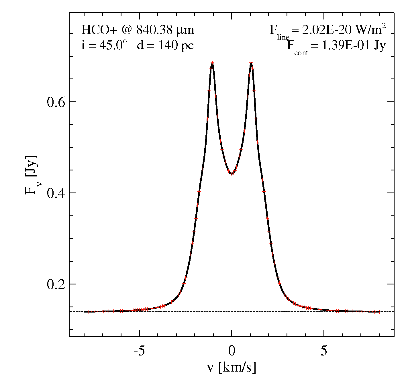
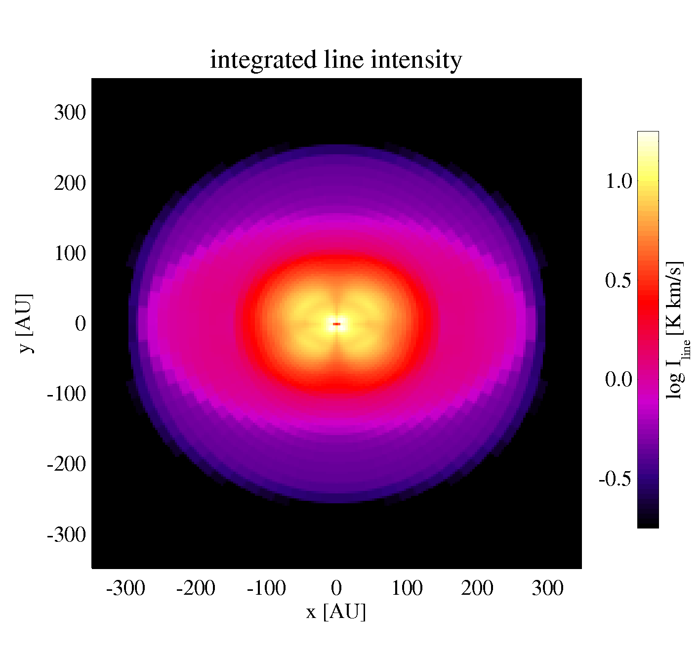
These outputs are similar to the main idl-output created by prodimo.pro, but this time taken from the regular-grid output.

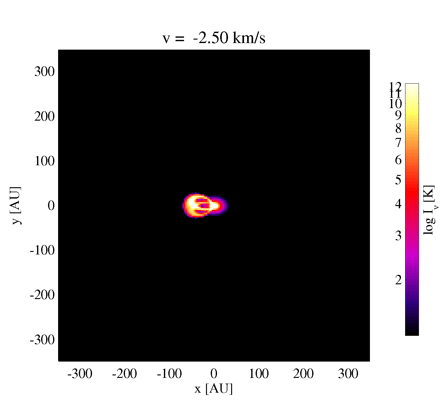
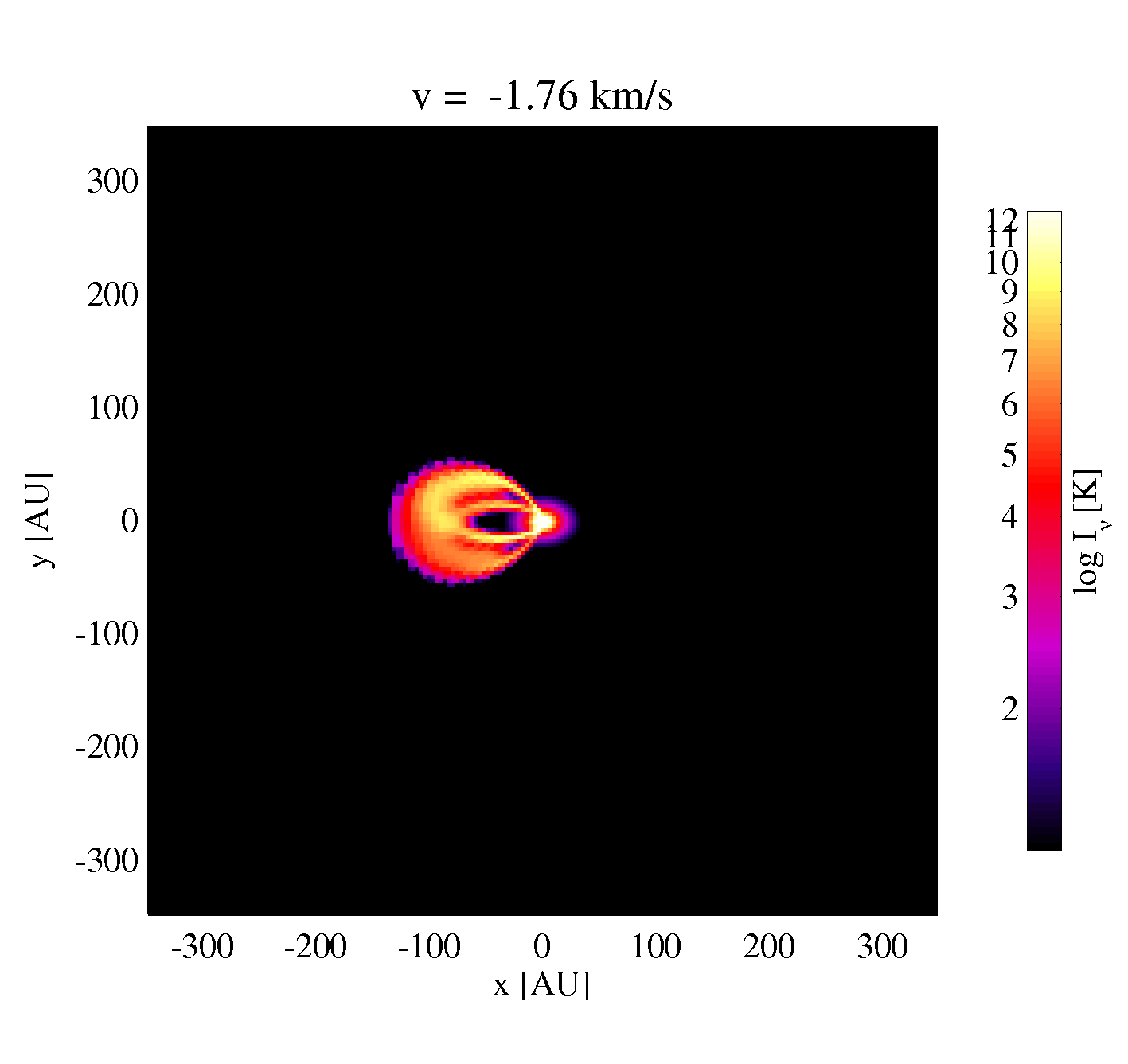
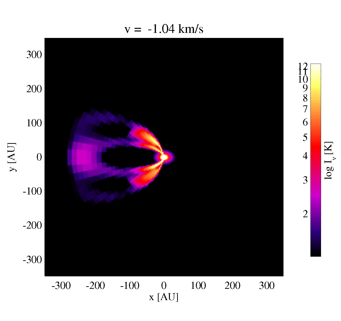
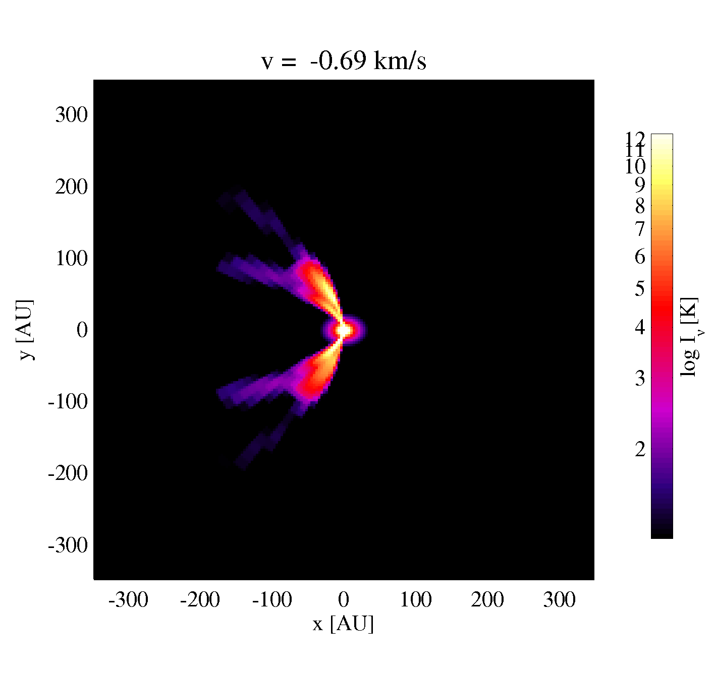
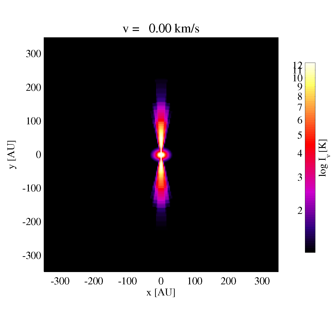
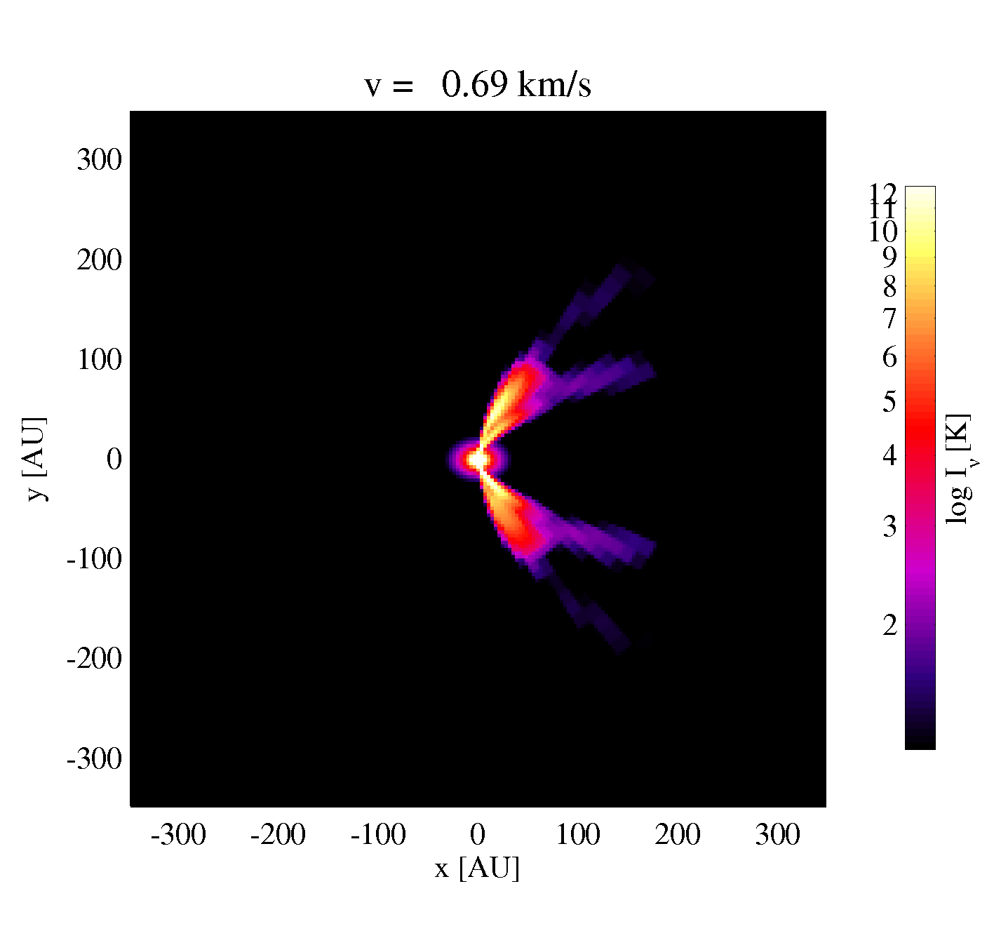
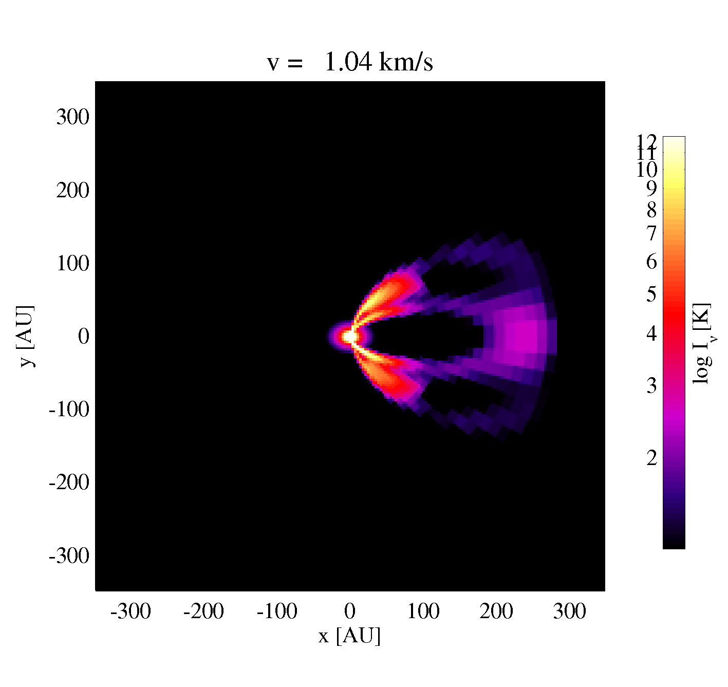
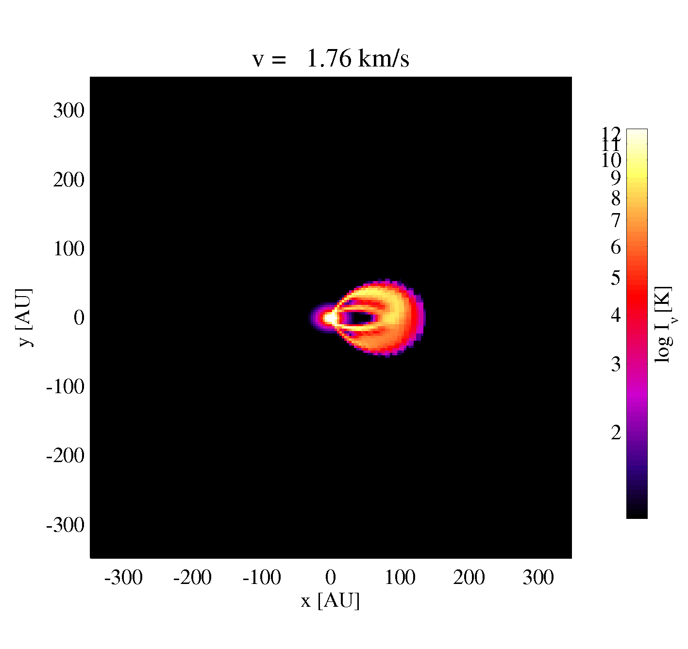
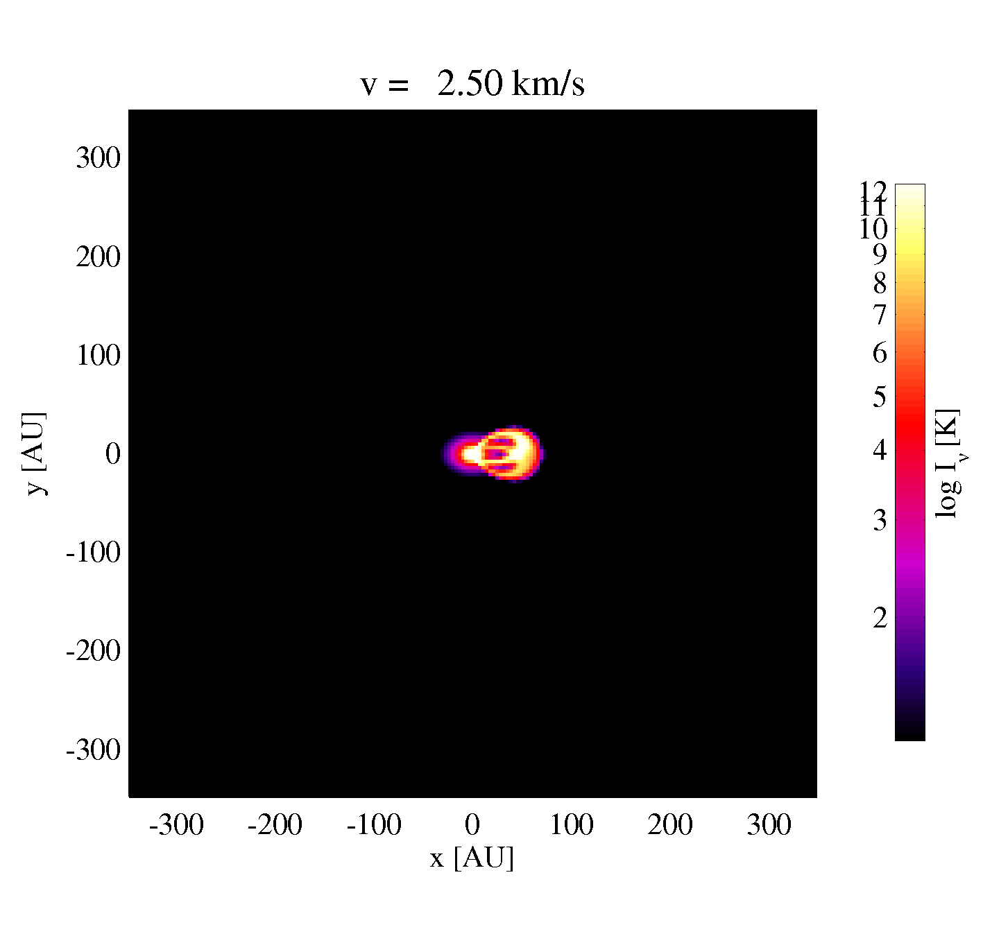
The channel maps are sorted by velocity. Each picture shows a double ring structure, one ring coming from the lower disk side, and the other coming from the upper disk surface. The lower disk ring may be missing if the dust is optically thick. For small velocities, the rings are open. For large velocities, the rings become small. For a pixel to be bright, there must be a point along the ray where the projected Keplerian velocity matches the observer's velocity, the molecule is abundant and excited.

Download a nicer version of the figures line3D.ps.gz.

Compiler option¶

From ProDiMo 2.0 the compiler option is not required anymore. For older versions, ProDiMo needs to be compiled with the compiler directive -DLINE_CUBE., to produce line cubes.