Parameter fitting
One the aims of ProDiMo is to provided an undestanding of actual protoplanetary discs. Therefore few fitting methods are now provided (for the moment specifically designed for parallele computers under the OAR software ([https://gforge.inria.fr/projects/oar/]). The current algorithm is the unicellular genetic algorithm in "evolution.f". I reproduce here the description given by Peter W. The Monte-Carlo Markov Chain method to compute parameter posterior distribution probabilities is discussed at the bottom of the page.
Genetic algorithm
P. Woitke:
I wrote a short program to do an automated chi-minimisation, including photometry-SED, Spitzer med-res spectrum, and observed line fluxes.
All necessary files can be found in input_examples/autofit if you update. As it stands, it will only run with ifort on FOSTINO, but with small modifications, it should be easy to make it running everywhere.
I use evolution strategy. A parent gets 8 children, each with slightly modified model-parameters. According to the principle "survival of the fittest", only the child with lowest chi-squared survives and becomes the new parent in the next generation. All other children die. This strategy is known to be very robust, it can escape small local minima, it can deal with very large number of parameters, and it can deal with noise in the chi-squared-determination. There may be better chi-squared-minimisation strategies though, so this is only a start ...
To use evolution.f, you first have to tell the program which parameters are to be varied. This is done in "Evo.in":
0      999      9           ! lastgen, maxgen, no.of parameters
1.0                         ! the step size
1.5E-3    0.15E-3   1  Mdisk
5.0E-5    0.50E-5   1  dust_to_gas
30.0      3.0       1  Rout
0.5       0.05      0  epsilon
0.008     0.0002    1  MCFOST_H0
1.12      0.01      0  MCFOST_BETA
0.05      0.005     1  amin
4.1       0.05      0  apow
0.03      0.003     1  fPAH
For each parameter, there is a starting value, a typical modification level, a switch whether to vary logarithmically(1) or linear (0), and the name.
You have to modify and copy Evo.in to your working folder. Also copy evolution.f and run.bsh to your working folder and type
$ cp ../input_examples/autofit/Evo.in .
$ cp ../input_examples/autofit/evolution.f .
$ cp ../input_examples/autofit/run.bsh .
$ ifort -o evolution evolution.f
There are new routines sed_chi.f and line_chi.f in ProDiMo which calculate chis with respect to observed fluxes in SEDobs.dat and (new) LINEobs.dat. The latter refers to the order in LineTransferList.in :
28/02/2013: New format for LINEobs.dat
If you want a summary of how good the predicted line fluxes and FWHM fit to the observed ones, you'll need another input file called LINEobs.dat which contains entries for line flux [W/m2], sigma_flux [W/m2], FWHM [km/s] and sigma_FWHM [km/s] as
0.0        1.7E-20    0.0    0.0   ul
30.5E-18   3.2E-18    0.0    0.0   ok
65.0E-18   25.E-18    38.0  10.0   ok
2.5E-18    0.1E-18    18.0   1.2   ok
Use "0.0 0.0" if FWHM is unknown. These informations are essential for automated fitting. The order of lines is the same as in '''LineTransferList.in".
Now, evolution creates folders like gen0001_child01, automatically fills them with all necessary input files, and then starts prodimo in these folders simultaneously by means of a script "run.bsh" for the FOSTINO cluster:
#!/bin/bash
#OAR -l /nodes=1/core=1,walltime=2:0:0
#OAR --name object_name_fit
#OAR --stdout prodimo.log
#OAR --stderr prodimo.err
ulimit -s unlimited
./prodimo
When the above input-files have been modified, just type
$ evolution > Evo.out &It currenty works with 8 children in every generation, i.e. 8 parallel jobs. evolution will wait until all jobs in one generation are ready, and then determine the fittest child. The combined (SED+Spitzer+line)-chi can be found in "finished.out" once a job is completed.
evolution runs for maxgen-lastgen generations, see above.
That's it - next day/week/month you can see how the chis have become smaller ...
$ grep "SED-chi" gen00?/prodimo.log
gen0001/prodimo.log: ==>        SED-chi =  0.5528
gen0002/prodimo.log: ==>        SED-chi =  0.4898
gen0003/prodimo.log: ==>        SED-chi =  0.4976
gen0004/prodimo.log: ==>        SED-chi =  0.5085
gen0005/prodimo.log: ==>        SED-chi =  0.4819
$ grep "Spitzer-chi" gen00?/prodimo.log
gen0001/prodimo.log: ==> Spitzer-chi = 0.7815
gen0002/prodimo.log: ==> Spitzer-chi = 0.7069
gen0003/prodimo.log: ==> Spitzer-chi = 0.7060
gen0004/prodimo.log: ==> Spitzer-chi = 0.7473
gen0005/prodimo.log: ==> Spitzer-chi = 0.7489$ grep "LINE-chi" gen00?/prodimo.log
gen0001/prodimo.log: ==> LINE-chi = 2.1912
gen0002/prodimo.log: ==> LINE-chi = 1.8672
gen0003/prodimo.log: ==> LINE-chi = 1.7532
gen0004/prodimo.log: ==> LINE-chi = 1.6084
gen0005/prodimo.log: ==> LINE-chi = 1.5811$ grep "chi" gen00?/finished.out
gen0001/finished.out: SED+LINE chi = 1.12625549339910
gen0002/finished.out: SED+LINE chi = 0.971908205746221
gen0003/finished.out: SED+LINE chi = 0.937039821553830
gen0004/finished.out: SED+LINE chi = 0.893458612093709
gen0005/finished.out: SED+LINE chi = 0.866576051357279... or how the parameters change values ...
$ grep "Rout" Evo.out
          Rout  T:  3.000E+01 3.000E+00
          Rout  2.6981E+01
          Rout  2.5864E+01
          Rout  2.5292E+01
          Rout  2.4133E+01
          Rout  2.3013E+01
Have fun,
Peter
Parallel Simplex fitting
Alternatively you can use the optimization program simplex_fit.f90, which is based on the Simplex method ([http://en.wikipedia.org/wiki/Simplex_algorithm]). The program was designed to run in parallel mode like evolution.f on the Fostino cluster. The basic paper explaining the parallel implementation is Lee & Wiswall 2007, Computational Economics, 30, p171-187: "A Parallel Implementation of the Simplex Function Minimization Routine". To use it, go to the directory where you have all the files to run a disk model:
$ cp ../input_examples/autofit/Simplex.in .
$ cp ../input_examples/autofit/m_mrgref.f90 .
$ cp ../input_examples/autofit/simplex_fit.f90 .
$ cp ../input_examples/autofit/run.bsh .
$ make -f makefile.simplex_fit
You have to modify the Simplex.in file
1 50 5 5 5
0.5 ! weigth_photometry
0.0 ! weight_Spitzer
0.5 ! weight_LINES
1e-5   0.1  1  Mdisk
1e-2   1.0  1  dust_to_gas
1e-2   1.0  1  fPAH
1.0    10   0  MCFOST_H0
0.5    5.0  1  MCFOST_BETA
The first line is simplex start number = 1, maximum number of simpexes = 50, number of parameters = 5, number of extra model per simplex >= number of parameters = 5, number of parallel runs usually =< number of parameters = 5. The weights are for the calculation of Chi like with evolution.f. The 5 next lines are for the parameters and their range. Example the line 1e-5 0.1 1 Mdisk means a lower bound of 1e-5, a upper bound of 0.1 and 1 means a log variation (0 means a linear variation) for the parameter Mdisk. In the example, MCFOST_H0 will be varied linearly.
To run the search, type from the model directory:
./simplex_fit > simplex.out &At the end of each Simplex run, the program writes the files vertices.out in the directory simple*, where (simplex0001) is the number of the run. The vertices.out* file contains in increasing chi value the parameters. The last column are the chi values.
The program chooses random values as starting point if the start number is 1. If you have a previous
run ending at simplex 24 (ie simplex0024/vertices.out) then you can restart the search by typing 24 50 5 5 5 in the first line instead.
The use of Simplex is good if you have no idea about the parameters. Start with large ranges and after a few runs, shrink the parameter search ranges to accelerate the optimization.
Simplex searches are very fast but since the runs are correlated, they cannot be used to provide an estimate of the parameter probability distributions. For that I suggest that you find first the best parameters with simplex_fit and then use evolution_mcmc.f for probe the parameter probability distributions.
Monte-Carlo Markov Chain
Monte-Carlo Markov Chain MCMC ([http://en.wikipedia.org/wiki/Markov_chain_Monte_Carlo]; [http://www.soton.ac.uk/~sks/utrecht/]) is a computational method that provides both a way to find a 'best fit' to observational data by a model with n parameters and a way to estimate the joint posterior probability distribution ([http://en.wikipedia.org/wiki/Posterior_distribution]) for each of the parameters, making it possible to undestand the uniquness and degeneracies in the parameters.
A state is a model. A Markov chain is a list of states; the parameters of each of them are related to the parameters of the previous state only ([http://en.wikipedia.org/wiki/Markov_chain]). The evolution.f code in /input_examples/autofit/ uses an algorithm that is actually a Markov Chain.
The Metropolis-Hasting method can be easily incorporated into the evolution mechanism ("evo_mcmc.f).
The program will produce a file name "evo_hist.out". The first columns are the parameters for each
best child-model and the last value is the chi-squared. The Metropolis-Hasting algorithm is used
to chose between a new generation and the current one:
-
if the best child (among the N children) is better than the parent (lower chi2) chose the child
-
if none of the child is better, throw a random number and compare it to the ratio between the likelihood of the best child and that of the parent. The likelihood is just the exp(chi2). If the random number is lower than the ratio, the new generation is accepted; otherwise new children are created from the same parent (in evolutionary term, the current offspring dies quickly..., the parent can have an other offspring).
In actual MCMC works, multiple chains should be try to ensure that the global minimum is actual reached.
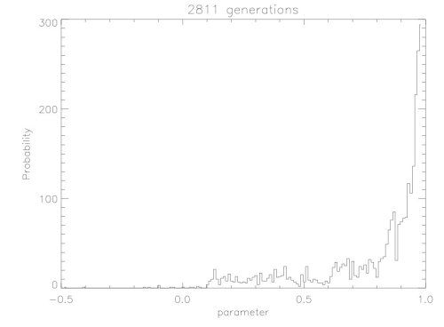
At equilibrium (ie close to the global minimum) the MCMC method will wander around, probing the parameter hypersurface. It is therefore possible to plot the parameter distributions (after binning the parameter in bins): the relative number of times a parameter is chosen. The absolute probabilties are not retrievable by this method but the moments are: peak probability, standard deviation, skewness, etc...
The only limitation is the noise in the joint posterior probability distributions because of the limited number of models (a model is relatively expensive to cumpute with ProDiMo). Also the method tends to avoid bad regions so that their statisitics are low for reconstructing the posterior probabilities.
A parameter distribution that is peaked with a small deviation means a paremeter that is well constrained by the observations while a quasi flat distribution means an unconstrained parameter. The following plot shows the probability distribution for one of the parameters generated by a MCMC version of evo_test.f name evo_mcmc.f. The maximum is at 1 but the method does not exactly reach this value. The distribution is however peaked with a narrow width at half-peak.