How to create a simple mid-IR line spectrum based on the line fluxes computed with escape probabilities?¶

By default, ProDiMo calculates all line fluxes with escape probability and outputs them into the file "FlineEstimates.out". In the src_develop folder, you will find a simple FORTRAN program that creates a high-resolution wavelength grid, puts all line fluxes on their best-maching wavelength points, and then convolves the spectrum to a given spectral resolution, for example R=2500. This "escape probability spectrum" can be used, e.g., for a rough comparison to a continuum-subtracted JWST spectrum. In order to create the output files that can later be visualised, run "eprospec" in your ProDiMo run-folder like this:

> cd src_develop
> gfortran -fdefault-real-8 -fdefault-double-8 eprospec.f -o eprospec
> cd MyRunFolder
> eprospec

which will create output files like these:

eprospec_C2H2_H.out
eprospec_CH4_H.out
eprospec_CO.out
eprospec_CO2_H.out
eprospec_H2.out
eprospec_H2O.out
eprospec_HCN_H.out
eprospec_NH3_H.out
eprospec_OH.out
eprospec_all.out
eprospec_ions.out

The output will depend on the molecules and lines included in your ProDiMo simulation. If you want additional molecules and different selection of lines, use a 'LineSelection.in' in your ProDiMo model. If you want a different wavelength range or different R, modify eprospec.f.

You can visualise the eprospec*.out yourself, or use this python code

> cd MyRunFolder
> python2 ~/ProDiMo/python/Plot_eprospec.py
> evince eprospec.pdf &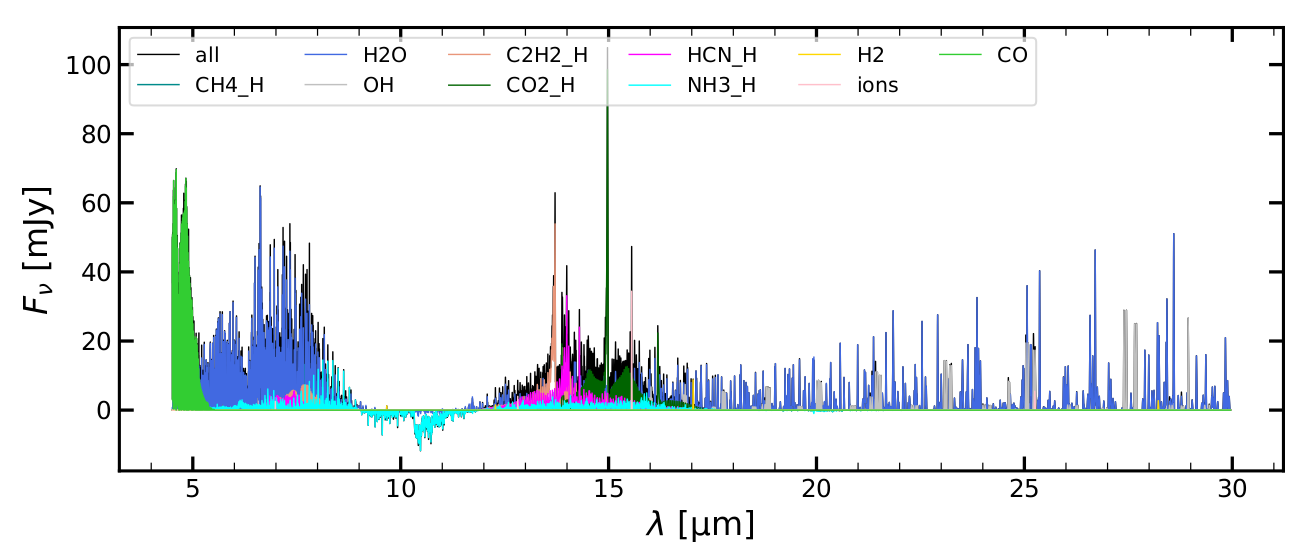

The screen output of Plot_eprospec.py lists some interesting integrated and line peak fluxes:

wavelength range [mic]:  4.9 8.0
molecules Fint[mJy*mic]    Fpeak[mJy]
    CH4_H      2.774906     17.190000
      H2O     20.127571     64.560000
       OH      0.000014      0.001479
   C2H2_H      1.731339      7.269000
    CO2_H      0.000000      0.000000
    HCN_H      1.825778      5.523000
    NH3_H      2.166184     10.080000
       H2      0.000738      0.204600
     ions      0.007412      2.492000
       CO      1.842529     40.900000

wavelength range [mic]:  13.0 17.7
molecules Fint[mJy*mic]    Fpeak[mJy]
    CH4_H      0.000000      0.000000
      H2O      5.321269     14.950000
       OH      0.443380      7.417000
   C2H2_H      9.818661     53.890000
    CO2_H      9.211376     98.530000
    HCN_H      6.897557     33.100000
    NH3_H      3.380544      4.953000
       H2      0.063390      8.735000
     ions      0.227837     34.400000
       CO      0.000000      0.000000

The example spectrum was created using the examples/StandardObjects/TTauri_new model which has settle_method=3, a_settle=0.001, and newUVphoto=3.

How to create a proper mid-IR line spectrum with FLiTs, based on the disk shape, dust opacities and line populations calculated by ProDiMo?¶

First, you need to download and compile FLiTs, the Fast Line Tracer by Michiel Min, see wiki FLiTs for a few details. It is important that you pass the multi=true argument when compiling to make it openmp-parallel:

> cd FLiTs
> make multi=true

Next, you need to run ProDiMo with the .true. ! FLiTs flag in your Parameter.in. This will create a number of "*.Lambda.dat" files and the main exchange file "ProDiMoForFLiTs.fits" or "ProDiMoForFLiTs.fits.gz" or "ProDiMoForFLiTs.dat".

Now you are all set to run your FLiTs simulations. In order to automatise, I use a csh-script called run.FLiTsQuick. To prepare running that script, we need to compile a fortran program that reads the output from FLiTs and then convolves the FLiTs spectrum to a given spectral resolution.

> cd src_develop
> gfortran -fdefault-real-8 -fdefault-double-8 flitsspec.f -o flitsspec

To further prepare running the script, you need the following input files for FLiTs: 'H2O_quick.in', 'OH_quick.in', 'C2H2_quick.in', 'HCN'_quick.in, 'CO2_quick.in', 'NH3_quick.in', 'CH4_quick.in', 'CO_quick.in', 'ions_quick.in', 'H2_quick.in', 'all_quick.in', and 'SO2_quick.in'. You can extract these files from this tar-file inputFLITS.tgz. You need to put these files in a directory as specified in run.FLiTsQuick, in my case it's ${HOME}/FLiTs/input.

Now you can run the script like this:

> cd MyRunFolder
> ./run.FLiTsQuick > FLiTs.log &

This takes about 30min on my Linux-PC. Once successfully run, you will find the following files in your MyRunFolder:

specFLiTs_C2H2.out
specFLiTs_CH4.out
specFLiTs_CO.out
specFLiTs_CO2.out
specFLiTs_H2.out
specFLiTs_H2O.out
specFLiTs_HCN.out
specFLiTs_NH3.out
specFLiTs_OH.out
specFLiTs_ions.out
specFLiTs_all.out
specFLiTs_conv_C2H2.out
specFLiTs_conv_CH4.out
specFLiTs_conv_CO.out
specFLiTs_conv_CO2.out
specFLiTs_conv_H2.out
specFLiTs_conv_H2O.out
specFLiTs_conv_HCN.out
specFLiTs_conv_NH3.out
specFLiTs_conv_OH.out
specFLiTs_conv_ions.out
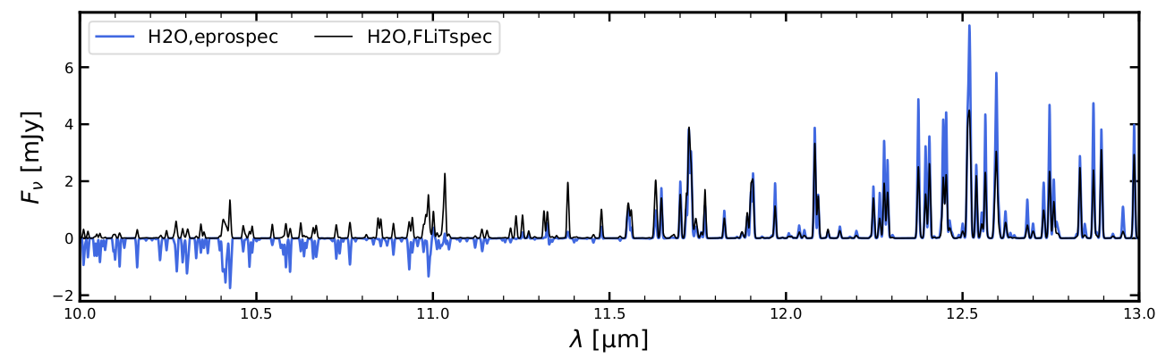
specFLiTs_conv_all.out

The specFLiTs_*.out are the FLiTs output spectra, and the specFLiTs_conv_*.out are the convolved spectra generated by flitsspec. Now we can visualise the latter, in comparison to the eprospec_*.out

> python2 ~/ProDiMo/python/Plot_eprospec_FLiTspec.py
> evince eprospec_FLiTspec.pdf &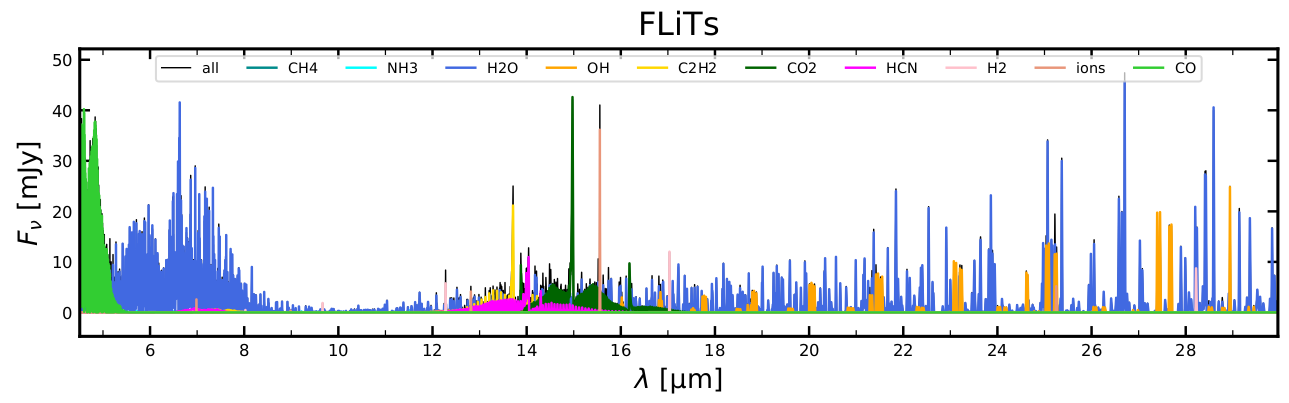

You will see some quite significant differences between the escape-probability-spectrum and the FLiTs-spectrum when you study the various eprospec_FLiTspec.pdf pages, for example the peak fluxes are almost a factor 2 lower, the FLiTs simulation does not confirm the NH3 absorption features as predicted by escape probability, etc. Some of the molecular emission lines are quite nicely predicted by escape probability, others are not.

Peter Woitke, Jan. 2025