Dust opacity parameters¶

Dust composition¶

To define the dust composition of a single dust grain, the following parameters have to be set in the Parameter.in file:

1      ! NDUST                  : number of selected dust species
1.0    AstroSilicate_Draine[s]  : volume fraction, dust species name

This will use the optical constants for the so called AstroSilicates and the dust grain consists only of this material.

Another (more realistic) example are the so called DIANA dust opacities composition:

3         ! NDUST           : number of selected dust species     
  0.60    Mg0.7Fe0.3SiO3[s] : volume fraction, dust species name
  0.15    amC-Zubko[s]
  0.25    vacuum[s]

which is a mixture of 3 dust species, where one is vacuum to simulate a porous grain. For more details see Woitke+ (2016).

ProDiMo includes a large sample of optical constants for various dust species, see Dust opacity data.

Size distribution¶

The dust size distribution is defined in the Parameter.in file with the following parameters:

0.05        ! amin        [mic]   : minimum dust particle size  
2000.0      ! amax        [mic]   : maximum dust particle size
3.5         ! apow        [-]     : dust size distr f(a)~a^-apow

For further details and examples of resulting dust opacities see also Woitke+ (2016).

Another relevant parameter is the dust size binning, which might has to be adjusted (increased) if you see unexpected artefacts in the resulting dust opacities.

300    ! NSIZE    : number of dust size bins

Please note the for larger NSIZE parameters the dust opacity calculations can take a long time, especially if the dust size distribution is broad (i.e. large amax/amin ratio). The default value is 300, which should be sufficient for most models. If you use hollow spheres, the default value is 80. If you just want to do some quick tests (i.e. explore different size distributions, compositions), lowering this values might be useful, to increase performance.

Size bin weighting¶

The way ProDiMo constructs the size distribution is explained in Section 4.6 of Woitke+ (2009). The integration of the size distribution is done from amin to amax. For example, the following Figure (left hand side panel, blue solid line) shows the normalize size distribution for amin=0.01, amax=1000 and apow=3.5. For simplicity we use only 6 size bins (NSIZE=6).

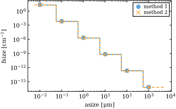
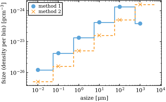
The horizontal line for each dust size (blue circles) indicate the width/weight (da) of the bin. This normalized distribution will give $\sum fsize(a)\times da= 1$ . The right-hand-side shows how this size distribution looks like when transformed to dust densities (for a given gas density, gas-to-dust ratio, and internal dust grain density).

The dashed orange line in both panels shows the same size distribution but with slightly different weights for amin and amax (i.e. the distance to the next smallest/largest grain size is considered). Both methods are fine, and method 1 remains the default. However, in some case the other method is also useful, in particular for interfaces to other codes, or for comparison. To activate method 2 simply use

2           ! dust_size_distribution : type of dust size distribution

Output¶

For verbose_level >=0 the resulting dust size distribution is also written to the files dust_fsize_rho.out and dust_fsize.out (normalized distribution). The file dust_sigmaa.out contains the vertical dust surface densities as a function of radius, per grain size. This file can be usefull to compare with 1D dust evolution codes (see also 1D Interface).

Mie calculations¶

The scattering and absorption efficiencies for compact spherical dust grains are calculated using the Mie theory for $x=2\pi a/\lambda$ for $x< 10^4$ ($a$: grain radius, $\lambda$: wavelength, $x$: size parameter). The Mie code distributed with ProDiMo is MIEX by Wolf, S. and Voshchinnikov, N. V. (2004), see also https://www.blogs.uni-kiel.de/star/miex/.

The outputs from that code can be compared to that of Bohren & Huffman (bhmie, Bruce Draine's version http://www.astro.princeton.edu/\~draine/scattering.html adapted for use in ProDiMo). with the switch is .true. ! check_Mie. The Bohren & Huffman code can also be used instead of MIEX by setting .true. ! bh_mie.

For x>1e4, a geometric optic code is the only option. (GOMsphere, Zhou, X., S. Li, and K. Stamnes, Applied Optics, 42 (21), 4295-4306, 2003). Note that a couple of bugs in the original version of GOMsphere have been corrected.

Size parameter¶

The GOMsphere code has problems with the calculation of the anisotropic factor g. It mainly produces noise and most of the calculation time actually is spent for the calculation of g. The MIEX code actually works also for size parameters x > 1.d4. Some tests have shown that it works fine up to x=1.d6, although it becomes very slow for this big size parameters. However, for a usual dust size distribution with grains up to $1000\,\rm \mu m$ it works just fine and is also faster than the GOMSphere code. With a the new parameter:

5.d5       ! sizeParam_Mie (default is 5.d5)

on can control up to witch x the MIEX code should be used.

This is also important for the dust opacities in the X-ray regime where the GOMSphere code has problems. But MIEX also cannot be used for the whole X-ray range as it becomes too slow and too memory demanding. The calculation of the scattering and absorption cross section is not a problem for the GOMSphere code in the X-ray range (and is also much faster), but the calculation for g does not work. So I changed the calculation of anisotropy factor g and replaced it by a simple approximate formula (which is mainly a fit to the MIEX results). This works fine for the X-ray regime. For small dust particles the Rayleigh-Gans approximation is now used (only for the X-ray regime!) as it is faster than the MIEX routine and the differences to the MIEX results are not significant.

The following figures show the pseudo anisotropic scattering cross sections (= (1-g)*isotropic scat cs) for various sizes and size distributions for Astronomical Silicates.

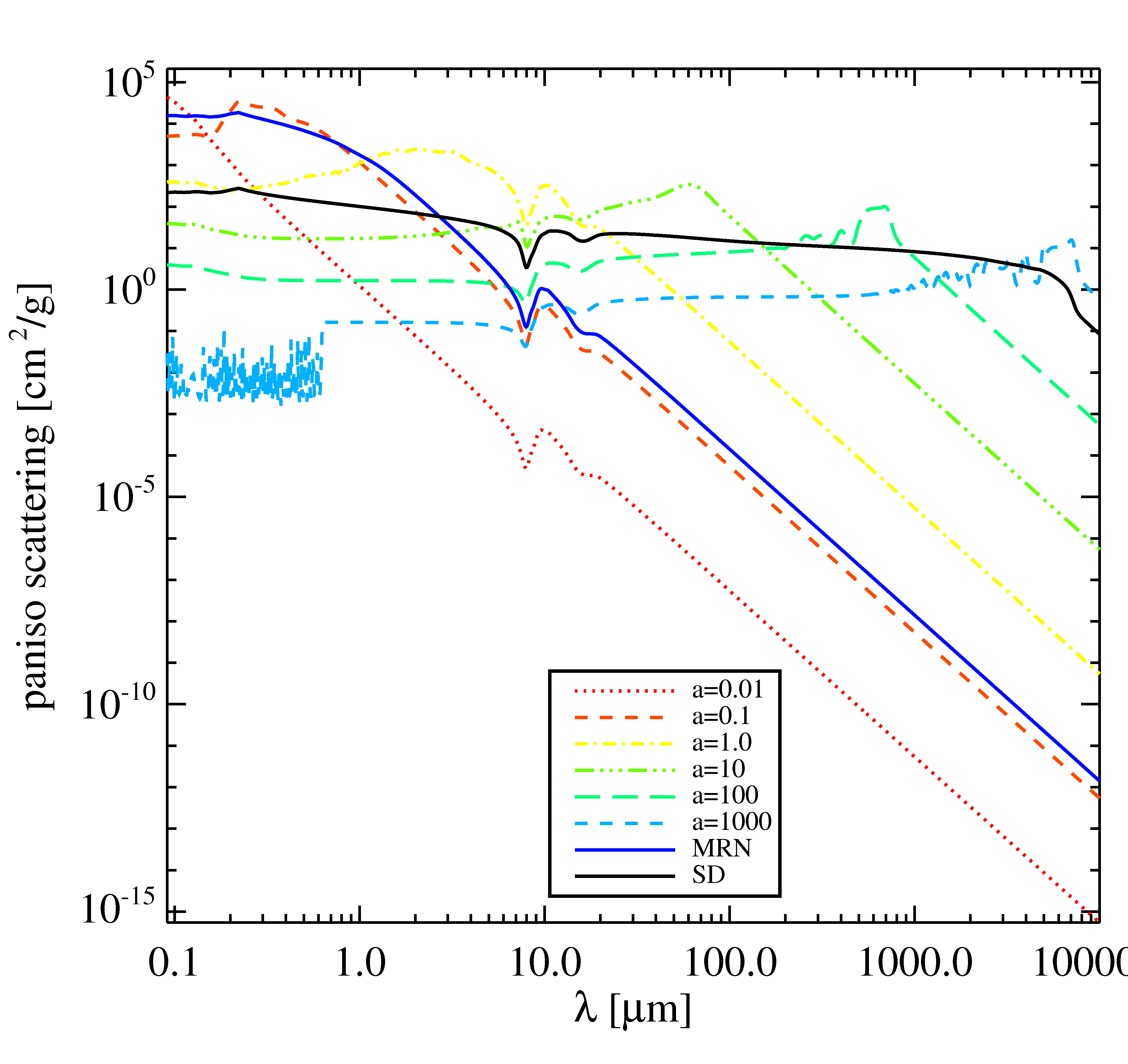
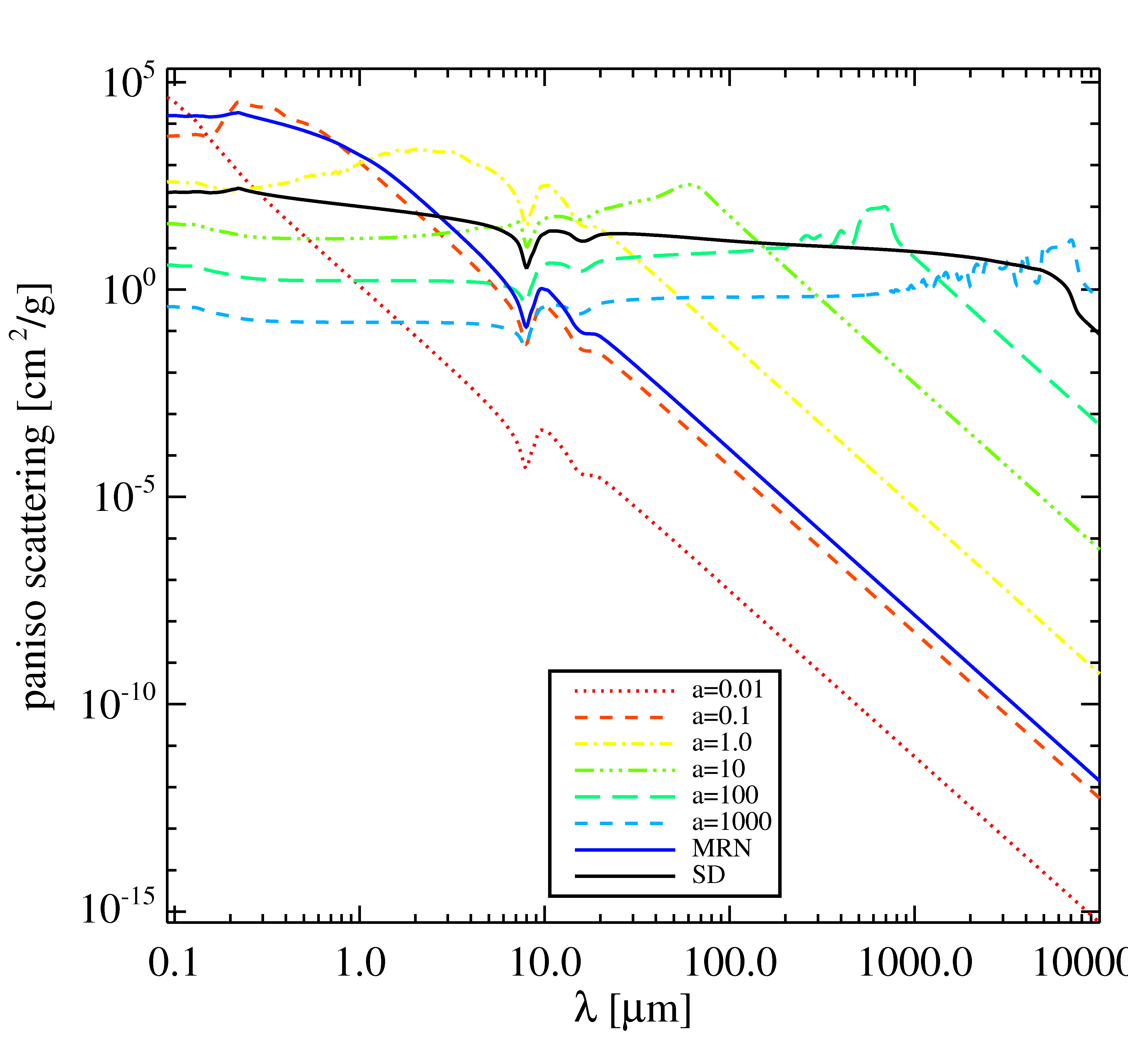
The left panel shows the results for the combination of MIEX and GOMsphere the right panel the results where only MIEX was used. Size distribution MRN: amin=0.005, amax=0.25, apow=3.5; size distribution SD: amin=0.01, amax=1000, apow=3.5

Porous grains¶

By default, the grains are compact in ProDiMo. Porous grain optical constants can be computed using the effective medium theory to compute porous grain opacities (see Li and Lunine 2003 ApJ 594 987; and Li and Lunine 2003 ApJ 598 51 for an astrophysical use). Porous grains are best used for transition/debris discs. The main effect is an enhanced millimetre/cm emissivity for a given solid mass. Porous grains with 90% vacuum was used by Li and Lunine to fit the SED of HD141596A. The following option in Parameter.in will compute a 90% porous grain with 10% crystallinity:

3        ! NDUST     [-]           : number of selected dust species
0.09    AstroSilicate_Draine[s]    : volume fraction and name of condensate
0.01    cryst_silicate[s]          
0.9     vacuum                     

Scattering cross sections¶

ProDiMo calculates both the absorption and scattering cross sections for the dust. However, due to the radiative transfer method used, the scattering cross-section is always the isotropic one (i.e. different to Monte Carlo Codes). However, one can use a simple approximation to take some effects of anisotropic scattering into account, by setting the parameter

.true.      ! pseudo_aniso_scat : use pseudo anisotropic scattering cross sections

The pseudo anisotropic scattering cross sections is given $(1-g)\times \rm isocs$, where $g$ is the anisotropy factor and isocs is the isotropic scattering cross section. For details and references see Rab+ 2018 and RT Benchmark.

Effective medium theory¶

The default effective medium theory is the Bruggeman model for spherical inclusions (see Bohren, C. F. & Huffman, D. R. 1983 - Absorption and scattering of light by small particles). There is an option to use the LLL model (Landau, L. D. & Lifshitz, E. M. 1960, Electrodynamics of continuous media, ed. Landau, L. D. & Lifshitz, E. M.; Looyenga, H. 1965, Physica, 31, 401):

.true. ! LLL     : use Landau, Lifshitz, Looyenga model

Reference: Tuncer+ 2005

The differences between the two formulations are negligible. A slight difference (a few percent) exists in the far IR to millimetre domain. Both formulations accept any volume fraction.

Other methods (Hunderi) and (Hunderi for a continuous distribution of ellipsoidal inclusions) are available Granqvist & Hunderi 1977

.true.  ! Hunderi

and

.true.  ! Hunderi_CDE

The classical Maxwell-Garnett method can be used as well

.true. ! Maxwell_Garnett

Hollow spheres¶

By setting the parameter

0.8     ! hollow_sphere   : use distribution of hollow spheres, 0.8 max hollow volume ratio (typical value)

to a value between 0.0 < volume ratio < 1, ProDiMo will compute the dust opacities using a distribution of hollow spheres. The idea is to "break" the symmetry in the calculation, which can introduce spurious solid features in the IR. The method was proposed by Min , Hovenier, and de Koter (2005) as a simple (i.e. easy to compute) alternative to the full calculation of distribution of randomly shaped grains. This option is best used simultaneously with a high wavelength sampling in the mid-IR.

The coated-sphere Mie code used is dmilay by Toon, O. B., and Ackerman, T. P. (1981)

If dmilay fails ProDiMo will use CMIEinstead (Cai+ 2010). One can also chose to only use CMIE by stetting:

.true.    ! c_mie    : Use the CMIE code instead of dmilay for hollow sphere calculations