Spectral Energy Distribution (SED)
By default, ProDiMo will calculate the SED at a distance of 140pc under 45 degree inclination, even if radiative_transfer=.false.. So, even if you have switched off proper radiative transfer, you will still get an impression about how your assumed dust temperature structure and dust size parameters would look like. You can adapt the settings for the SED calculation by adding the following lines to your Parameter.in:
------ image and SED parameters ------
.true.      ! calcSED            : calculate SED and images?
200         ! NlamSED            : number of lambda gridpoints
0.2         ! lminSED            : minimum lambda[mic]
5000.0      ! lmaxSED            : minimum lambda[mic]
97.0        ! dist      [pc]     : distance
45.0        ! incl      [deg]    : inclination (0=face-on)
.true.      ! write_image_out    : Produce image for each wavelength (image.out) ?
SED calculation can be switched off by setting calcSED=.false.
Use NlamSED to choose the number of wavelength points (maximum 75000, but that will be slow) and lminSED (micron) and lmaxSED (micron) to specify the wavelength range. ProDiMo will use a logarithmically equidistant wavelength grid in between. The opacity will be interpolated at the ProDiMo wavelength values.
Set dist and incl to change distance (in pc) and inclination (in degrees with 0 being a disk seen face-on). The incl parameter also accepts multiple values:
0,20,40,80 ! incl [deg] : calculate SED for the given inclinations.By default the SED calculations also produce an image for each wavelength point (see Continuum Images). However, such a file can become quite big, and if not needed this can be switched off by setting write_image_out=.false.-
To switch to an older mode for SED calculation (using the spectral bands from the continuum RT) you can use monoSED=.false.. However, this is only recommended if you want to rerun very old models monoSED=.true. is the default and recommended value.
User-defined wavelength grid
In some cases, it is useful to have the results from the SED calculations at distinct wave-length points defined by the user (e.g. exactly at those points where I have observational data). This can be done by providing a file called SEDlamgrid.in. If this file is found in the current model directory, ProDiMo calculates the SED only at the wavelength points given in that file. An example of such a file is attached (SEDlamgrid.in). The unit for the wavelength is micron.
Comparing with observations
The idl-macro prodimo.pro (but also the prodimopy python tools) will visualize the spectral flux (SED) and the spatial distribution of continuum intensity (images) at several wavelengths. It will also look for a file called SEDobs.dat that is supposed to contain all observational photometric data to compare the calculated SED with. Format is as
29
  lam[mic]     Flam[Jy]     sigma[Jy]  rem  filter    Ref
     0.155     0.252941     0.017433    ok  generic   Wesselius et al.(1982)
     0.180     0.434248     0.028122    ok  generic   Wesselius et al.(1982)
     0.220     0.489273     0.037767    ok  generic   Wesselius et al.(1982)
     0.249     0.720323     0.049025    ok  generic   Wesselius et al.(1982)
     0.329     1.517713     0.067827    ok  generic   Wesselius et al.(1982)
    11.5      28.763314     1.728675    ??  IRAS12    Weaver & Jones(1992)
    24.0      49.598494     3.965399    ??  IRAS25    Weaver & Jones(1992)
    65.0     115.504082    11.552718    ??  IRAS60    Weaver & Jones(1992)
   105.0     114.368223    11.440253    ??  IRAS100   Weaver & Jones(1992)
   350.002     8.927684     1.409592    ok  generic   Mannings(1994)
   449.997     3.819208     0.569864    ok  generic   Mannings(1994)
   749.998     0.526936     0.080990    ok  generic   Mannings(1994)
   800.000     0.504942     0.045995    ok  generic   Mannings(1994)
   850.000     0.358966     0.066994    ok  generic   Mannings(1994)
  1100.000     0.149987     0.020998    ok  generic   Mannings(1994)
  1300.000     0.102993     0.017999    ok  generic   Mannings(1994)
  2700.000     0.010599     0.000400    ok  generic   Mannings(1994)
 0.344         1.7948       3.4243E-01  ok  Stroemgren_u      Vizier catalogue
 0.410         5.5029       5.0755E-01  ok  Stroemgren_v      Vizier catalogue
 0.467         5.8944       2.4286E-01  ok  Stroemgren_b      Vizier catalogue
 0.550         5.5035       2.0280E-01  ok  Stroemgren_y      Vizier catalogue
 0.365         2.8112E+00   2.5892E-03  ok  Johnson_U_Turpol  Benjamin
 0.43          5.7099E+00   5.2590E-03  ok  Johnson_B_Turpol  Benjamin
 0.55          5.4784E+00   5.0458E-03  ok  Bessell_V         Benjamin
 0.63          5.2155E+00   9.6072E-03  ok  Coussins_R        Benjamin
 0.78          4.5600E+00   8.3999E-03  ok  Coussins_I        Benjamin
 1.25          6.7223E+00   1.1145E-01  ok  J_2Mass    Cohen(2003)
 1.65          9.8599E+00   1.8164E-01  ok  H_2Mass    Cohen(2003)
 870.0         0.00895      0.0116      ul  LABOCA     Neal(2009)
The first three columns are lambda[micron], flux[Jy] and sigma[Jy]. 4th column is a flag: ok = valid observational data (point), ul = upper limit (point with downward arrow), ?? = unused observation (smaller point), UL = unused upper limit. Note that sigma is 1-sigma, even for upper limits. Unused means that this point is disregarded in the computation. The 5th column contains the names of the filter transmission files. "filter-name" means that ProDiMo will take the transmission data from ProDiMo/data/filter/filter-name.dat.
If you compile your SEDobs.dat, you need to know, for every point, which platform and instrument were used, and find the according filter transmission file somewhere, which you should add to /ProDiMo/data/filter. From the calculated model fluxes Fnu(lambda), ProDiMo will then integrate over lambda, weighted by that filter transmission, to calculate a flux in [Jy] that can be compared to the observational value provided in this file. If you have only magnitudes, you have to convert the magnitudes to Jansky. If you want to do this correctly, you need to know the "zero-point" of the instrument-filter-combination, I actually do not know how to do that properly. Otherwise, just use http://www.stsci.edu/hst/nicmos/tools/conversion_form.html, where you need to know, however, at least the central wavelength of the filter. It can make quite a difference, for example, whether it's filter "R" or "Rs"! If the filter name is specified as "generic", a generic filter profile is generated with 12% spectral width, or 1% for "mono".
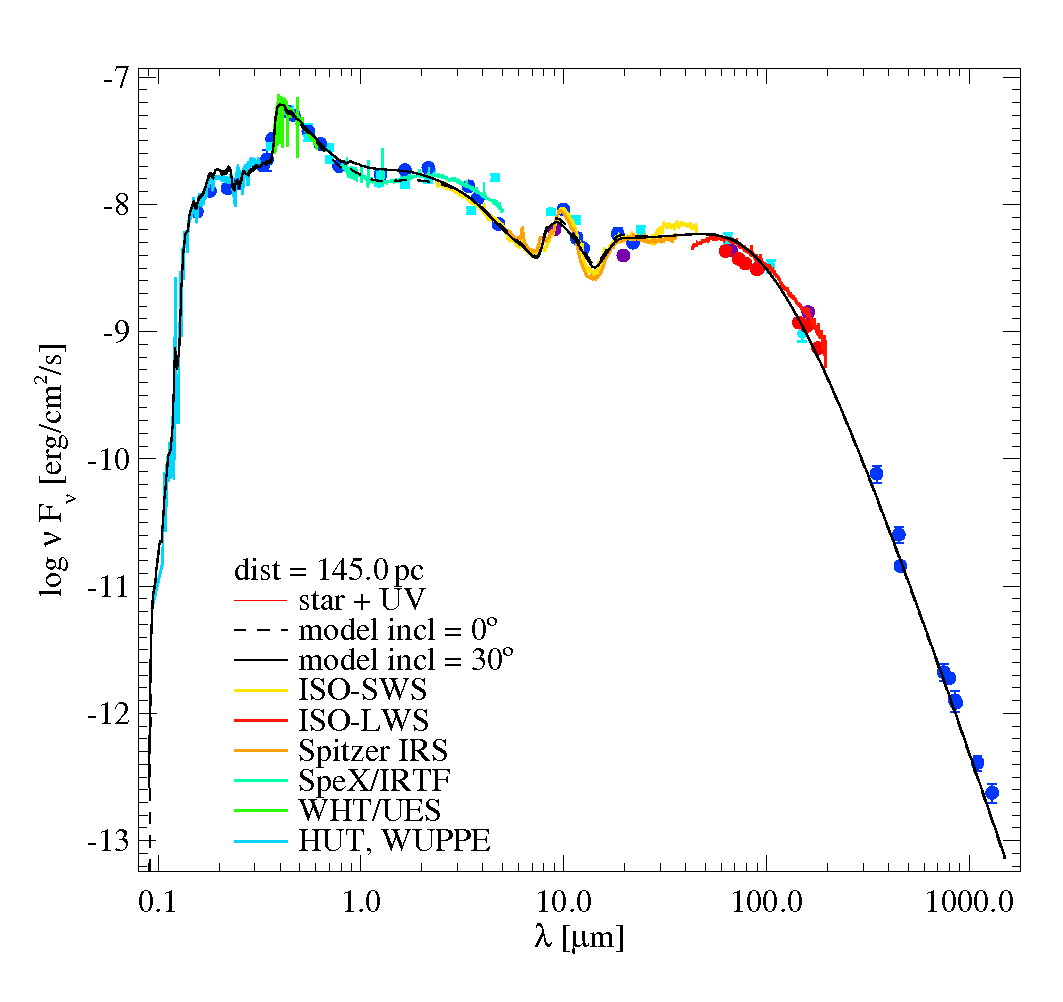
If you have done everything correctly, prodimo.pro will visualize the calculated SED, and observations, in a plot like this. Besides the used (blue) and unused (cyan) photometric points, ProDiMo and prodimo.pro will automatically read low-resolution spectra from
UV.dat                  lam[A]   flux[erg/cm^2/s/A]    sigma
OpticalSpectrum.dat     lam[A]   flux[erg/cm^2/s/Hz]
nearIR_Spectrum.dat     lam[A]   flux[W/m2/mic]
SpitzerIRSspec.dat      lam[mic] flux[Jy]              sigma
ISO-SWS-spectrum.dat    lam[mic] flux[Jy]
ISO-LWS-spectrum.dat    lam[mic] flux[W/cm^2/mic]
if present. ProDiMo will then calculate two , first separately for photometry "chi_PHOTO", and all (near-far)-IR spectra "chi_SPITZER". You will find these chi-values in the stdout-file, for example, this model has
  ==> photometry-chi =  1.3890
  ==>    Spitzer-chi =  1.0397
There are two more chi, namely for the gas emission lines (see input_and_output_files), and for images (see Images). The overall quality of a model, in terms of how bad it compares to all available observations, is then calculated as
chi^2 = (  weight_PHOTO * chi_PHOTO^2 + weight_SPITZER * chi_SPITZER^2
         + weight_LINES * chi_LINES^2 + weight_IMAGES  * chi_IMAGES^2 )
      / ( weight_PHOTO + weight_SPITZER + weight_LINES + weight_IMAGES )
where the weights can be specified in Parameter.in, otherwise they are by default =1/4. In cases where no spectral, line or image data is present, the corresponding weights will be put to zero.
MCFOST-like SED chi2
25 March 2013 Revision 0b4a7f27
There is not a unique fool-proof way to compute chi-squared. The switch:
.true. ! chi_logbinwill group photometric points into bin in the log10 scale from 1 micron. For example, if there are 4 photometric points between 10 and 100 microns, each of those photometric band will be given a weight of 0.25. The stellar photometric data are not binned (lambda<1 micron). At the end, the chi-squared is normalized by the number of log10 bins. It is up to the user to test what is the best chi-squared computation for his/her problem. If the photometric points are well spaced in log10(wavelength) then the standard and the log10 binned chi-squared values should be similar. If there is a clustering of points in a given bin, this bin may have too much weight in the standard chi-squared computation. Here is an example:
    lam[mic]    Fmodel[Jy]  Fphot[Jy]        err
      0.1264 ok  1.717E-03  1.321E-03      0.615  generic
      0.1477 ok  2.319E-03  3.200E-03     -2.147  generic
      0.1679 ok  2.973E-03  2.326E-03      1.591  generic
      0.1894 ok  3.750E-03  2.658E-03      2.294  generic
      0.2196 ok  5.008E-03  5.736E-03     -0.904  generic
      0.2530 ok  6.631E-03  8.051E-03     -1.294  generic
      0.2863 ok  8.486E-03  1.054E-02     -1.447  generic
      0.3600 ok  1.446E-02  3.150E-02     -5.188  generic
      0.4400 ok  5.334E-02  6.760E-02     -1.580  generic
      0.5500 ok  1.621E-01  1.400E-01      0.979  generic
      0.7100 ok  3.511E-01  2.600E-01      2.002  generic
      0.9700 ok  6.376E-01  4.100E-01      2.944  generic
      1.2350 ok  7.808E-01  7.000E-01      0.728  generic
      1.6620 ok  9.571E-01  8.500E-01      0.791  generic
      2.1590 ok  7.287E-01  7.200E-01      0.080  generic
     10.8000 ok  6.067E-01  5.800E-01      0.300  generic
     12.0000 ok  5.785E-01  7.000E-01     -1.271  generic
     23.6800 ok  1.564E+00  2.270E+00     -2.484  generic
     25.0000 ok  1.686E+00  2.440E+00     -2.464  generic
     60.0000 ok  4.453E+00  3.920E+00      0.850  generic
     70.0000 ok  4.857E+00  3.903E+00      1.458  generic
     71.4300 ok  4.903E+00  3.640E+00      1.485  generic
    100.0000 ok  5.640E+00  5.040E+00      0.750  generic
    155.9000 ok  6.410E+00  6.570E+00     -0.123  generic
    160.0000 ok  6.441E+00  7.388E+00     -0.914  generic
    450.0000 ok  3.981E+00  4.250E+00     -0.327  generic
    800.0000 ok  1.963E+00  1.450E+00      1.416  generic
    850.0000 ok  1.770E+00  1.380E+00      1.659  generic
   1100.0000 ok  1.021E+00  8.740E-01      1.040  generic
   3400.0000 ok  9.696E-02  4.100E-02      5.738  generic
   7000.0000 ok  1.119E-02  8.000E-03      2.239  generic
The standard method gives: SED-chi = 2.0150 whereas the log10 binned chi-squared gives 1.9620.