Image Calculation and Image Processing
By default (if calcSED=.true.in Parameter.in) ProDiMo calculates formal solutions of the continuum radiative transfer on a bundle of parallel rays through the model disk, to compute the SED. The rays are organized in about 150 log-equidistant rings, and 72 equidistant angular points. As a side-result, this intensity-data can be visualized as images though IDL with prodimo.pro, for example ...
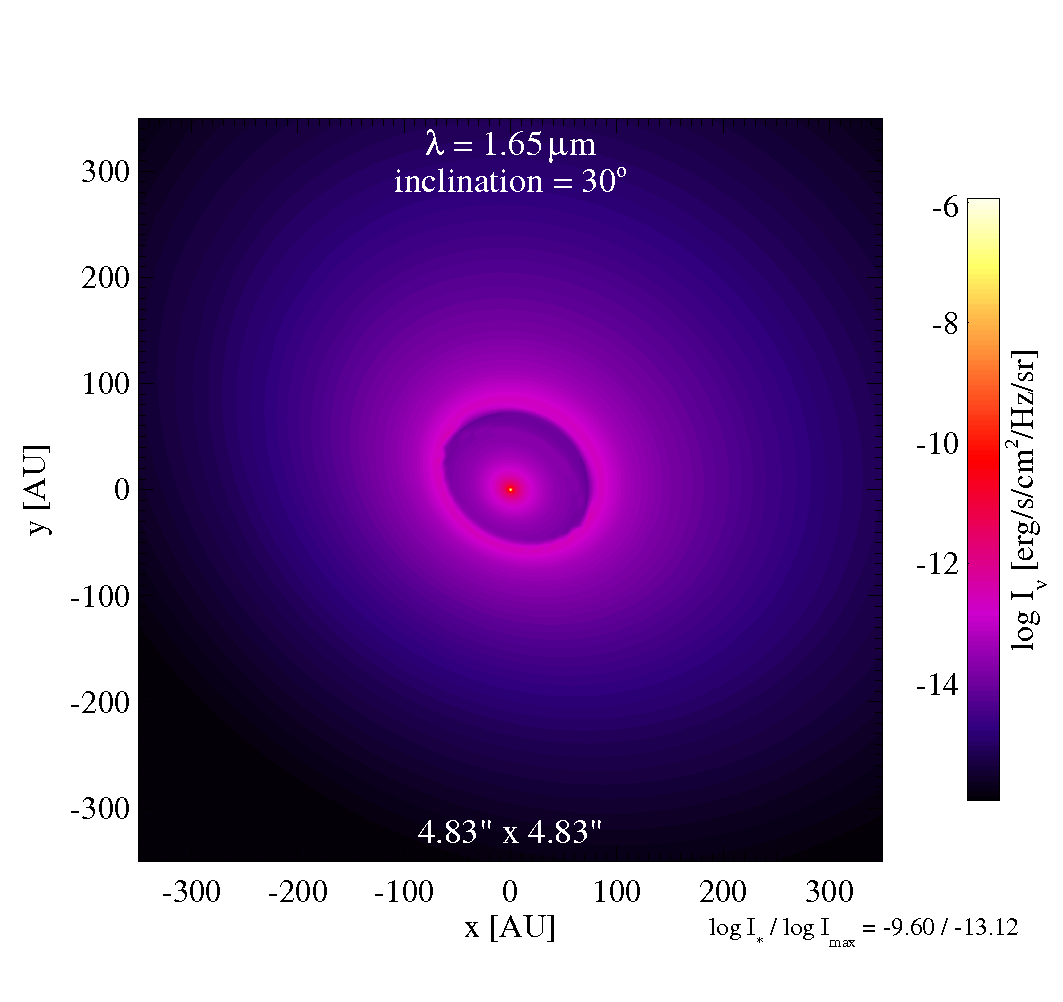
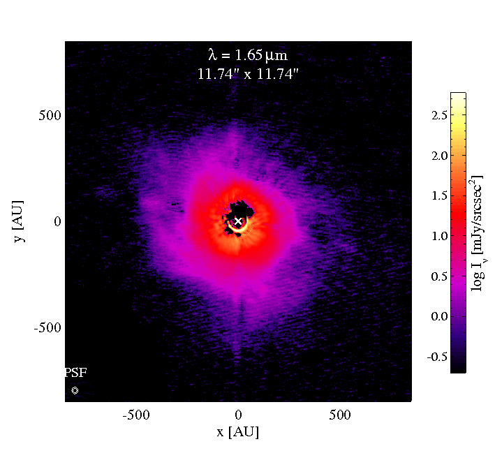
Left is the raw model image, right is an H-band observation of ABAur (Fukagawa 2004).
BE WARNED: PRODIMO CAN ONLY DO ISOTROPIC SCATTERING! Due to the preferred forward-scattering by large grains, the far disk side usually appears less bright then the front side. This it not realistically represented with ProDiMo. In the SED-computation this effect cancels out, more or less, so the SEDs calculated by ProDiMo are quite accurate, but a pixel-to-pixel comparison of image data is difficult.
We therefore restrict ourselves to the comparison of radial intensity profiles , which are averaged over angle. From the observational image fits-files, we calculate mean values and standard deviations of the intensities found in the image in certain radial bins with respect to the "center". Now, the same procedure is carried out with the model image, and then we can compare. However, we need to carefully simulate the procedure how the observational image data was obtained and post-processed, as precisely as possible. That involves
- spectral filtering,
- turn image into object's sky orientation
- PSF convolution,
- auto-center,
- PSF-subtraction,
(r) determination, and chi2-calculation.
In order to make ProDiMo do this, there is a specific input-file called image.in which reads as
ProDiMo input file for image processing
=======================================
3                         ! Nimage
30.0                      ! object position angle on sky
1.12     1.65    872.0    ! central wavelength [mic]
0.090    0.127   1.544    ! PSF bmin [arcsec]
0.090    0.127   2.037    ! PSF bmaj [arcsec]
0.0      0.0    -82.71    ! PSF position angle
F        F       T        ! auto-center?
T        T       F        ! PSF-subtraction?
60.0     125.0   50.0     ! Rin_valid [AU]
9999.9   9999.9  800.0    ! Rout_valid [AU]
generic
H_2Mass                   ! filter names
mono
Iprofile_NICMOS.dat
Iprofile_Hband.dat        ! observational intensity profiles
Iprofile_SMA.dat
The first line tells ProDiMo to create 3 images, and the second line is the disk's sky orientation (clockwise turn). Next come the center wavelengths and PSF ("beam")-properties of the respective instruments, where bmin is the PSF FWHM [arcsec] of the minor axis and bmaj is the PSF FWHM of the major axis. PSF position angle turns that pattern (here counter-clockwise by 82 degree) from upward orientation. The next two lines specify whether or not the image should be auto-centered, and PSF-subtracted. Then you can specify the radial range [AU] where the comparison to the observational profile is to be carried out. A similar syntax is used for LINEobs.dat where you can add observations of line intensity profiles, see an example in the lower part of input_and_output_files.
Next come the names of spectral transmission filter-files, same as in SEDobs.dat. The first step of the image processing is actually the simulation of the filter, so, at every point of the image, the available intensities as function of lambda are integrated over, weighted by the filter transmission. If specified as "generic", a generic filter profile is generated with 12% spectral width, or 1% for "mono".
If the auto-center option is activated, the position of the "image-center" will be determined by looking for the maximum in the convolved image, below a circular Gaussian with 5% angular width of image. The radial profile is then calculated with respect to this point.
Finally, the names of the input files containing the observational intensity profiles are specified. These files contain r[AU], [erg/s/cm2/Hz/sr] and sigma_Inu.
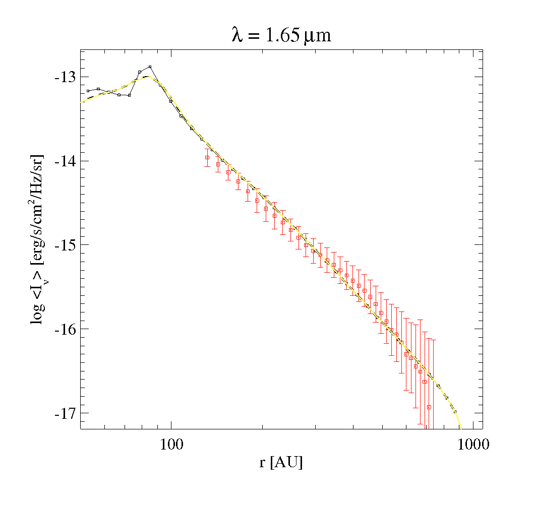
Full black line, and points, is the raw (un-processed) model profile, back-dashed and yellow lines are post-processed model profile (calculated in two different ways), and red are the observations.
Parameters for the raytracing/image grid
The number of radial and azimuthal points/rays used to create the images can be controlled via Parameter.in. This example shows the default values:
150         ! cont_Ndisk     grid points for the disk itself
4           ! cont_Nstar     for the star
40          ! cont_Nhole     between star and the disk
30          ! cont_Npuff     around the puffed up inner rim
72          ! cont_Ntheta    azimuthal directions
Continuum images for post-processing
For many cases, post-processing of images is required to make a direct comparison to observations. One common example is post-processing with CASA, to compare the model to ALMA observations. For that case an image format with regular/quadratic pixels is required. With the parameters
551        ! Npixel_continuum
.true.     ! continuum_cube_fits
images for each wavelength considered in the SED calculation, with 551x551 quadratic pixels, are created. All images are written to a single fits file called image.fits. The fits file can, for example, be viewed directly or post-processed with CASA.
If continuum_cube_fits=false (default), the images are written in a proprietary ASCII format into image.out.
If a high number of pixels is required (e.g. high spatial resolution observations) the image cube can be quite big. In that case, we recommend to use a user-defined wavelength grid (SEDlamgrid.in, see ProDiMo_SED) for the SED and image calculations. With SEDlamgrid.in it is possible to exactly define those wavelengths that are actually relevant for the comparison to observations. Be aware that in that case also, the SED is only calculated for the wavelength points given in SEDlamgrid.in.
There is also an option to limit the size of the resulting image. This is useful for example of having a better resolution without needing a huge number of pixels. The parameter is
100.0 ! cont_Rout outer radius consider for the image in auThis limits the FOV to 200 au, and all the pixels are used for that area only. This works in that same way as for Line cubes.