Input and Output files
TODO: Not up-to-date anymore, needs revision!
Input files
There are currently up to 7 input files to control what ProDiMo will do
Elements.in
Species.in
Reactions.in
Parameter.in
StarSpectrum.in
LineTransferList.in
image.in
The first 4 input files are compulsory, the other 3 can be added for special purposes. In addition, other input files are required when advanced options are used.
The files are in ascii and human-readable. They can be edited by any word editor. However, one should always use space and not TAB when formatting an input file as TAB will not be recognised by the code.
Elements.in, Species.in and Reactions.in
specify the chemical model in terms of element abundances, selection of gas-phase and ice species, and reaction rates beyond UMIST. There are two ways of specifying input abundances for all species. Either positive values behind the species in the file Species.in - see below - or negative ones. In the latter case, the negative values are taken as logarithmic initial abundances for each species and the user has to ensure that they add up to the desired element abundance. The code will calculate the element abundance from them and overwrite Elements.in.
If values are positive, a "1.0" denotes where the total abundance for that element found in Elements.in is put. For example, set C+ to 1.0 means that the code will start with all the carbon in the species C+ and other species containing the carbon element should be very low ().
One can also choose to distribute it over the ions, but not over molecules. To prevent the user from erroneously choosing positive values that do not add up to 1, the code will stop when it finds that the element abundance calculated in Species.in deviates by more than 1% from that specified in Elements.in.
237
H        1.E-20
H+       1.0
H-       1.E-20
H2       1.E-20
H2+      1.E-20
H3+      1.E-20
H2exc    1.E-20
He       1.E-20
He+      1.0
HeH+     1.E-20
C        1.E-20
C+       1.E-20
C++      1.0
CH       1.E-20
CH+      1.E-20
The Reactions.in is not mandatory. If none is present in the model directory, ProDiMo take a default one: data/ChemicalNetwork/Reactions.in.csv.
Parameter.in
is the central parameter input file, where all physical, stellar, dust and disk parameters are specified. There are also parameters to control the computational grid, various switches where you can turn on/off different assumptions and options, and numerical parameters. The choice of the physical parameters is easy to understand by looking at one example file.
StarSpectrum.in
is optional where you can fix the stellar input spectrum. For historical reasons, the file should contain 12 lines of text and then lambda [nm] and the surface Eddington flux . Otherwise (if the file is not present), ProDiMo takes a PHOENIX spectrum of matching and (2D interpolation at every wavelength), and solar abundances.
LineTransferList.in
controls the parameter for ProDiMo's in-build line transfer, for example the choice of spectral lines. It needs to be there if line_transfer=.true. in Parameter.in. See details under ProDiMo Line Transfer.
image.in
has the parameters for calculation of images, post-processing like convolution with simulated instrument PSF, and comparison to observations, see Images for details.
Providing observational data
In addition to the *.in-files, there are *.dat files which contain various observational data the model will be compared to.
extinct.dat
SEDobs.dat
nearIR_Spectrum.dat
SpitzerIRSspec.dat
ISO-SWS-spectrum.dat
ISO-LWS-spectrum.dat
LINEobs.dat
Iprofile_NICMOS.dat
Iprofile_Hband.dat
Iprofile_SMA.dat
Iprofile_CO32.dat
LineProfile_CO32.dat
The names of the first 7 files are fixed. If these files exist, ProDiMo will automatically calculate several chi2 to assess the deviations between the model and the observations, in terms of photometric observations, low-resolution spectra, line observations and images. The values of these chi2, named chi_PHOTO, chi_SPITZER, chi_LINES, chi_IMAGES in the code, will appear in the stdout-file. A summary thereof, total_chi, will also be written to finished.out.
extinct.dat
contains the extinction parameters E(B-V) and Rv. SEDobs.dat contains photometric observations, as well as the names of filter extinction curve data-files, see ProDiMo_SED for an example.
Spectra
The following 4 files contain low-resolution spectral data: nearIR_Spectrum.dat has lambda[A] and flux[W/m2/micron], SpitzerIRSspec.dat has lambda[micron] and flux[Jy], as well as ISO-SWS-spectrum.dat. ISO-LWS-spectrum.dat, however, has lambda[micron] and flux[W/cm2/micron]. ProDiMo will automatically try to read these files, adding together all low-resolution spectral data, and then evaluate the deviation chi_SPITZER between the model SED and these spectra.
LINEobs.dat
contains observational data about gas emission lines, namely flux[W/m2], sig_flux[W/m2], FWHM[km/s] and sig_FWHM[km/s]. Use 0 0 if line width is unknown. The order of lines must be the same as in !LineTransferList.in, so the first input line corresponds to the first spectral line computation. If observed velocity-profiles F_nu(v) and/or radial intensity profiles
> more LineTransferList.in
number of lines, number of velo-points
5  151
upper level, lower level, vmax[km/s], name of molecule
2   1   10.0  OI
3   2   10.0  OI
2   1    6.0  CII
19  18  20.0  CO
4   3    6.0  CO
4   3    6.0  CO_lte
The last entry in the example will ask ProDiMo to generate a line flux and profile assuming a LTE population. The comparison between the CO and CO_lte outputs help in understanding the level of departure from LTE. The two first columns are the indices of the upper and lower levels (see the file !LineList.out for a correspondence to the actual level wavelengths). In the example the line ray-tracing will be performed between -vmax and vmax in steps of dv= 2 vmax/151 km/s. the number of velo-points should be an odd number to include the v = 0 km/s. As a simple rule of thumb, the sampling dv should be lower than the disk turbulent width set in Parameter.in.
> more LINEobs.dat
7.50E-16    8.1E-18     0.0   0.0   ok
3.26E-17    3.0E-18     0.0   0.0   ok
5.09E-17    2.0E-17     0.0   0.0   ok
2.96E-17    3.0E-18     0.0   0.0   ok
1.03E-18    2.0E-19     3.0   1.0   ok
--- line flux profiles ---
F       F       F       F       T        ! line profile available?
F       F       F       F       T        ! auto-center?
0.0     0.0     0.0     0.0     99.9     ! v_valid
nodata
nodata
nodata
nodata
LineProfile_CO32.dat
--- intensity profiles ---
30.0                                     ! object position angle on sky
F       F       F       F       T        ! intensity profile available?
F       F       F       F       T        ! auto-center?
0.0     0.0     0.0     0.0     1.671    ! PSF bmin [arcsec]
0.0     0.0     0.0     0.0     2.034    ! PSF bmaj [arcsec]
0.0     0.0     0.0     0.0    -84.63    ! PSF position angle
0.0     0.0     0.0     0.0     30.0     ! Rin_valid
0.0     0.0     0.0     0.0     900.0    ! Rout_valid
nodata
nodata
nodata
nodata
Iprofile_CO32.dat
In this example, there are spectral and angular resolved observations available for the CO 3-2 line, in data-files LineProfile_CO32.dat and Iprofile_CO32.dat. The comparison to an observational intensity-profile is particularly tricky, since the model intensity map needs to be convolved with the PSF of the instrument first. More infos about the image processing is here Images.
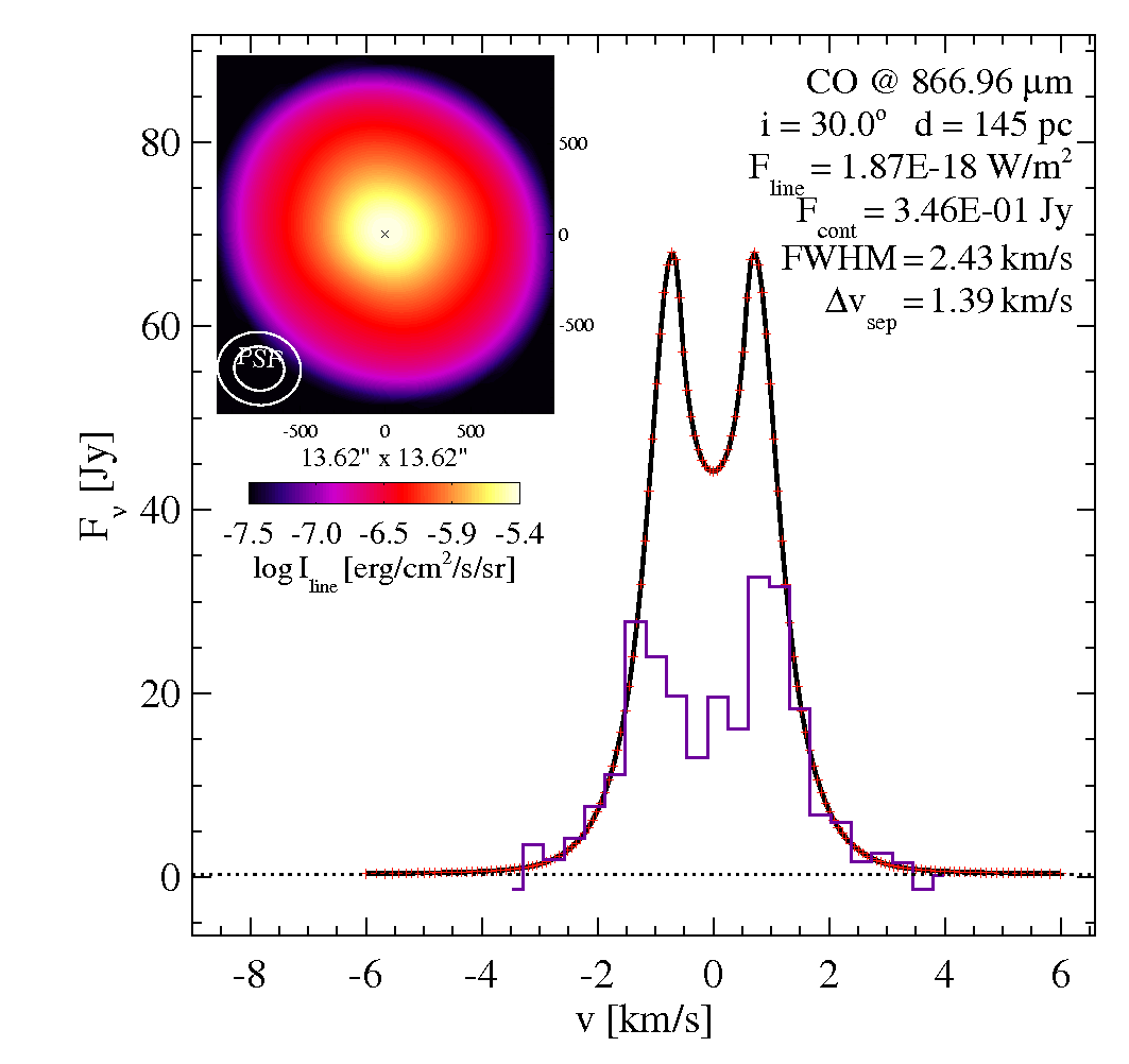
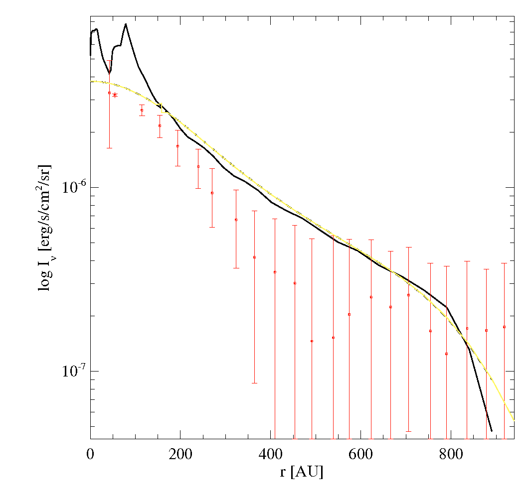
In this case, the CO line seems to be too bright (too much flux AND too high intensities at given radius), and too extended (from velo-separation as well as from intensity profile).
Output files
The standard output-files are
  Elements.out         : summary of elemental abundances
  Species.out          : summary of selection of species
  Reactions.out        : complete list of chemical reactions compiled from different sources
  ChemInit.log         : log-file for chemical initialization process
  LineList.out         : summary of spectral lines included

  ProDiMo.out          : main output file, contains all physical, chemical and radiative properties (r,z)
  dust_opac.out        : dust opacities in cm^2^/g(dust) lambda[mic]  kext  kabs   ksca
  RTinterpolation.out  : data to see how good the spline-interpolation in lambda works
  StarSpectrum.out     : stellar spectrum lamb[mic] and Inu[erg/cm2/s/Hz/sr]
  FlineEstimates.out   : estimation of all gas emission lines fluxes, directly using
  finished.out         : total time consumption, and total chi
  Parameter.out        : a summary of all the flags/switches
In addition, there will be additional output files created, if certain options are activated
  SED.out              : computed continuum fluxes, twice, for face-on and for specified inclination angle
  image.out            : computed image data
  image_conv_??.out    : computed image data convolved with instrument PSF
  Iprofile_*.out       : mean continuum and line intensities as function of radius, after convolution

  line_flux.out        : computed line flux and velo-profile data, from line transfer
  line_image.out       : computed Iline(x,y) from line transfer
  LINE_3D_???.out      : full 3D-cube outputs for channel maps
  LINE_COVERAGE.out    : achieved quality of pixel coverage thereof

  pop_LTE_*.out        : fractional LTE population of all atomic/molecular species on grid
  pop_PRO_*.out        : fractional population as calculated from escape probability in ProDiMo
  PAH_cross.out        : the PAH cross-section used in your model
Almost all output files can be automatically visualized with the main idl-macro prodimo.pro. In addition, there are more idl-macros for special purposes and also prodimopy for plotting with Python, see Look_at_the_results.
Optional output
A detailed chemical reaction output can be requested by switch a flag in the Parameter.in file. See chemistry_details.